![]()

Tutorial 1: Un/Self-supervised learning methods#
Week 3, Day 3: Unsupervised and self-supervised learning
By Neuromatch Academy
Content creators: Arna Ghosh, Colleen Gillon, Tim Lillicrap, Blake Richards
Content reviewers: Atnafu Lambebo, Hadi Vafaei, Khalid Almubarak, Melvin Selim Atay, Kelson Shilling-Scrivo, Jiaxin Cindy Tu
Content editors: Anoop Kulkarni, Spiros Chavlis
Production editors: Deepak Raya, Gagana B, Spiros Chavlis, Konstantine Tsafatinos
Tutorial Objectives#
In this tutorial, you will learn about the importance of learning good representations of data.
Specific objectives for this tutorial:
Train logistic regressions (A) directly on input data and (B) on representations learned from the data.
Compare the classification performances achieved by the different networks.
Compare the representations learned by the different networks.
Identify the advantages of self-supervised learning over supervised or traditional unsupervised methods.
Setup#
Install dependencies#
Show code cell source
# @title Install dependencies
# @markdown Downloads the dataset, checkpoints, and images needed for this
# @markdown tutorial. The module code is inlined in the hidden cells below.

import os, shutil
from io import BytesIO
from urllib.request import urlopen
from zipfile import ZipFile

REPO_PATH = "neuromatch_ssl_tutorial"
download_str = "Downloading"
if os.path.exists(REPO_PATH):
    download_str = "Redownloading"
    shutil.rmtree(REPO_PATH)

zipurl = 'https://osf.io/download/69f4f21a33e868da65fe593d/'
print(f"{download_str} and unzipping... Please wait.")
with urlopen(zipurl) as zipresp:
    with ZipFile(BytesIO(zipresp.read())) as zfile:
        zfile.extractall(REPO_PATH)
print("Download completed!")
Downloading and unzipping... Please wait.
Download completed!
Module: Plot utilities#
Show code cell source
# @title Module: Plot utilities

import copy

from matplotlib import pyplot as plt
from matplotlib import colors as mplcol
import numpy as np


def add_annotations(image, annotations=None, center=None, color=None):
    """
    - annotations (str): If not None, annotations are added to images,
        e.g., 'posX_quadrants'. (default: None)
    - centers (list): If not None, centers are provided to annotate the
        images, in form [image_centers, image_double_centers], where
        image_centers and image_double_centers are iterables. (default: None)
    """

    image = copy.deepcopy(image)

    HEI, WID = 64, 64
    BUFFER = 16
    X_SPACING = 11
    N_QUADS = 3
    RADIUS = 2

    hei, wid = image.shape
    rel_hei = hei / HEI
    rel_wid = wid / WID

    x_buffer = int(np.around(rel_wid * BUFFER))
    y_buffer = int(np.around(rel_hei * BUFFER))

    if color is None:
        color = np.max(image) * 2

    if annotations is not None:
        if annotations not in ["pos", "posX_quadrants"]:
            raise ValueError(
                "If not None, annotations must be 'pos' or 'posX_quadrants'."
                )

        x_spacing = int(np.around(rel_wid * X_SPACING))

        # create dash square
        dash_len = 3
        hei_dash, wid_dash = [np.concatenate(
            [np.arange(i, v, dash_len * 2) for i in range(dash_len)])
            for v in [hei - y_buffer * 2, wid - x_buffer * 2]]

        image[y_buffer + hei_dash, x_buffer] = color
        image[y_buffer + hei_dash, wid - x_buffer] = color
        image[y_buffer, x_buffer + wid_dash] = color
        image[hei - y_buffer, x_buffer + wid_dash] = color

        # add dashed quadrant lines
        if annotations == "posX_quadrants":
            for n in range(1, N_QUADS):
                image[y_buffer + hei_dash, x_buffer + x_spacing * n] = color

        if center is not None:
            if len(center) != 2:
                raise ValueError(
                    "Expected 'centers' to have length 2, but found length "
                    f"{len(center)}."
                    )

            if np.max(center) > 1 or np.min(center) < 0:
                raise ValueError("Expected 'center' coordinates to be "
                    "between 0 and 1, inclusively.")

            # obtain coordinates in pixels
            quadrant_width = wid - 2 * x_buffer
            quadrant_height = hei - 2 * x_buffer
            x_center = int(np.around((center[0] * quadrant_width + x_buffer)))
            y_center = int(np.around((center[1] * quadrant_height + y_buffer)))

            radius_adj = (np.mean([rel_hei, rel_wid]) * RADIUS)

            xx, yy = np.mgrid[: image.shape[0], : image.shape[1]]
            circle = (xx - x_center) ** 2 + (yy - y_center) ** 2
            image[np.where((circle < (radius_adj ** 2)).T)] = color


    return image


def plot_dsprites_images(images, ncols=5, title=None, annotations=None,
                         centers=None):
    """
    plot_dsprites_images(images)

    Plots dSprites images.

    Required args:
    - images (array-like): list or array of images (allows None values to
        skip subplots). If each image has 3 dimensions, the first is assumed
        to be the channels, and is
        averaged across.

    Optional args:
    - ncols (int): maximum number of columns. (default: 5)
    - title (str): plot title. If None, no title is included. (default: None)

    Returns:
    - fig (plt.Figure): figure
    - axes (plt.Axes): axes
    """

    # average channel dimension
    for i, image in enumerate(images):
        if image is not None and len(image.shape) == 3:
            images[i] = np.mean(image, axis=0)

    num_images = len(images)
    ncols = np.min([num_images, ncols])
    nrows = int(np.ceil(num_images / ncols))
    fig, axes = plt.subplots(nrows=nrows, ncols=ncols,
        figsize=(ncols * 2.2, nrows * 2.2), squeeze=False
        )

    if title is not None:
        fig.suptitle(title, y=1.04)

    if annotations is None:
        color_list = ['black', 'white']
    else:
        color_list = ['black', 'white', 'red']

    if centers is None:
        if annotations is not None:
            centers = [None] * len(images)
    elif len(centers) != len(images):
            raise ValueError(
                "If providing centers, must provide as many as the number "
                "of images."
            )

    cmap = mplcol.LinearSegmentedColormap.from_list(
        'dsprites_cmap', color_list, N=len(color_list))

    for ax_i, ax in enumerate(axes.flatten()):
        if images[ax_i] is not None and ax_i < num_images:
            image = images[ax_i]
            if annotations or centers:
                image = add_annotations(
                    image, annotations=annotations, center=centers[ax_i]
                    )
            ax.imshow(image, cmap=cmap, interpolation='nearest')
            ax.set_xticks([])
            ax.set_yticks([])
        else:
            ax.axis('off')

    return fig, axes


def plot_dsprite_image_doubles(images, image_doubles, doubles_str, ncols=5,
                               title=None, annotations=None, centers=None):
    """
    plot_dsprite_image_doubles(images, image_doubles, doubles_str)

    Plots dSprite images is sets of 2 rows.

    Required args:
    - images (list): list of images
    - image_doubles (list): list of image doubles (same length as images)
    - doubles_str (str or list): string that specified what the doubles are,
        or list if specifying both images and image_doubles.

    Optional args:
    - ncols (int): number of columns. (default: 5)
    - title (str): plot title. If None, no title is included. (default: None)
    - annotations (str): If not None, annotations are added to images,
        e.g., 'posX_quadrants'. (default: None)
    - centers (list): If not None, centers are provided to annotate the
        images, in form [image_centers, image_double_centers], where
        image_centers and image_double_centers are iterables. (default: None)

    Returns:
    - fig (plt.Figure): figure
    - axes (plt.Axes): axes
    """

    if len(images) != len(image_doubles):
        raise ValueError(
            "images and image_doubles must have the same length, but have "
            f"length {len(images)} and {len(image_doubles)}, respectively."
            )

    if not isinstance(images, list) or not isinstance(image_doubles, list):
        raise ValueError("Must pass images and image_doubles as lists.")

    plot_centers = None
    if centers is not None:
        if len(centers) != 2:
            raise ValueError("centers must be of length 2 with center values "
                "(or None) for the images and image_doubles."
            )

        for s, sub_centers in enumerate(centers):
            if sub_centers is None:
                centers[s] = [None] * len(images)
            elif not isinstance(sub_centers, list):
                raise ValueError(
                    "Centers must comprise 2 lists: one for images and one "
                    "image_doubles (or None in either position)."
                    )
            elif len(sub_centers) != len(images):
                raise ValueError(
                    "Must provide as many values as images/images_double."
                    )

        plot_centers = []

    plot_images = []
    ncols = np.min([len(images), ncols])
    n_sets = int(np.ceil(len(images) / ncols))
    for i in range(n_sets):
        use_slice = slice(i * ncols, (i + 1) * ncols)
        extend_images = images[use_slice]
        extend_image_doubles = image_doubles[use_slice]

        padding = [None] * (ncols - len(extend_images))

        plot_images.extend(
            extend_images + padding + extend_image_doubles + padding
            )

        if plot_centers is not None:
            extend_image_centers = centers[0][use_slice]
            extend_image_double_centers = centers[1][use_slice]
            plot_centers.extend(
                extend_image_centers + padding +
                extend_image_double_centers + padding
            )

    fig, axes = plot_dsprites_images(
        plot_images, ncols=ncols, annotations=annotations, centers=plot_centers
        )
    fig.tight_layout()
    if title is not None:
        fig.suptitle(title, y=1.04)

    images_str = "Images"
    if isinstance(doubles_str, list):
        if len(doubles_str) != 2:
            raise ValueError("If 'doubles_str' is a list, it must be of length 2.")
        images_str, doubles_str = doubles_str

    x_left = axes[0, 0].get_position().x0
    x_right = axes[-1, -1].get_position().x1
    x_ext = (x_right - x_left) / 30
    for r, row_start_ax in enumerate(axes[:, 0]):
        ylabel = images_str if not r % 2 else doubles_str
        row_start_ax.set_ylabel(ylabel)

        if r != 0 and not r % 2:
            top_ax_y = axes[r - 1, 0].get_position().y0
            bot_ax_y = axes[r, 0].get_position().y1
            y = np.mean([bot_ax_y, top_ax_y])

            line = plt.Line2D(
                [x_left - x_ext, x_right + x_ext], [y, y],
                transform=fig.transFigure, color="black"
                )
            fig.add_artist(line)

    return fig, axes


def plot_RSMs(rsms, titles=None):
    """
    plot_RSMs(rsms)

    Plots representational similarity matrices.

    Required args:
    - rsms (list): list of 2D RSMs arrays.

    Optional args:
    - titles (list): title for each RSM. (default: None)

    Returns:
    - fig (plt.Figure): figure
    - axes (plt.Axes): axes
    """

    if not isinstance(rsms, list):
        rsms = [rsms]
        titles = [titles]

    if len(rsms) != len(titles):
        raise ValueError("If providing titles, must provide as many "
            "as the number of RSMs.")

    min_val = np.min([rsm.min() for rsm in rsms] + [-1])
    max_val = np.max([rsm.max() for rsm in rsms] + [1])

    ncols = len(rsms)
    wid = 5

    fig, axes = plt.subplots(
        ncols=ncols, figsize=[ncols * wid, wid], squeeze=False
        )
    fig.suptitle("Representational Similarity Matrices (RSMs)", y=1.05)

    cm_w = 0.05 / ncols
    fig.subplots_adjust(right=1-cm_w*2)
    cbar_ax = fig.add_axes([1, 0.15, cm_w, 0.7])

    for ax, rsm, title in zip(axes.flatten(), rsms, titles):
        im = ax.imshow(rsm, vmin=min_val, vmax=max_val, interpolation="none")
        ax.set_title(title, y=1.02)

    cbar = fig.colorbar(im, cax=cbar_ax)
    cbar.set_label(label="Similarity", size=18)
    cbar_ax.yaxis.set_label_position("left")

    return fig, axes
Module: Data utilities#
Show code cell source
# @title Module: Data utilities
import os
import warnings
import numpy as np
import torch
from torch import nn
import torchvision
DEFAULT_DATASET_NPZ_PATH = os.path.join("dsprites", "dsprites_subset.npz")
def get_biased_indices(dataset, indices, bias="shape_posX", control=False,
randst=None):
"""
get_biased_indices(dataset, indices)
Returns indices after removing those rejected given the requested bias.
For example, if the bias is 'heart_right', the indices of any images where
the heart is on the right are removed.
Required args:
- dataset (torch dSprites dataset): dSprites torch dataset
- indices (1D np array): dataset image indices
Optional args:
- bias (str): way to bias the dataset subset defined by the indices.
'heart_left': only include hearts on the left
'shape_posX': correlate shape to posX
(default: "heart_left")
- control (bool): if True, the same number of items are excluded, as
determined by the bias, but they are randomly selected.
(default: False)
- randst (torch Generator or int): random state to use when splitting
dataset. (default: None)
Returns
- indices (1D np array): indices retained
"""
if bias == "heart_left":
shapes, pos_Xs = dataset.dSprites.get_latent_values(
indices, latent_class_names=["shape", "posX"]
).T
heart_value = dataset.dSprites.shape_name_to_value_map["heart"]
exclude_bool = ((shapes == heart_value) * (pos_Xs > 0.5))
elif bias in ["shape_posX", "shape_posX_spaced"]:
shapes, posXs = dataset.dSprites.get_latent_values(
indices, latent_class_names=["shape", "posX"]
).T
exclude_bool = np.zeros_like(indices).astype(bool)
shape_vals = dataset.dSprites.latent_class_values["shape"]
posX_vals = np.sort(dataset.dSprites.latent_class_values["posX"])
if bias == "shape_posX":
posX_val_splits = np.array_split(posX_vals, len(shape_vals)) # unequal split allowed
elif bias == "shape_posX_spaced":
posX_val_edges = [[0, 0.3], [0.35, 0.65], [0.7, 1.0]]
posX_val_splits = [[
val for val in posX_vals if val >= edges[0] and val < edges[1]
] for edges in posX_val_edges]
for shape_val, pos_valX_split in zip(shape_vals, posX_val_splits):
exclude_bool += (
(shapes == shape_val) * ~np.isin(posXs, pos_valX_split)
)
else:
raise NotImplementedError(
f"{bias} bias is not implemented. Only 'heart_left' and "
"'shape_posX' biases are currently implemented."
)
if control: # randomly permute the exclusion boolean
if isinstance(randst, int):
randst = torch.random.manual_seed(randst)
exclude_bool = exclude_bool[
torch.randperm(len(exclude_bool), generator=randst)
]
indices = indices[~exclude_bool]
return indices
def subsample_sampler(sampler, fraction_sample=1.0, randst=None):
"""
subsample_sampler(sampler)
Required args:
- sampler (SubsetRandomSampler): dataset sampler
Optional args:
- fraction_sample (float): fraction of sampler indices to retain in
new sample.(default: 1.0)
- randst (torch Generator or int): random state to use when subsampling.
(default: None)
Returns:
- sub_sampler (SubsetRandomSampler): subset dataset sampler (unseeded)
"""
if 1 <= fraction_sample <= 0:
raise ValueError(
"fraction_sample must be between 0 and 1, inclusively, but "
f"found {fraction_sample}."
)
subset_size = int(fraction_sample * len(sampler.indices))
if isinstance(randst, int):
randst = torch.random.manual_seed(randst)
sampler_indices = sampler.indices[
torch.randperm(len(sampler.indices), generator=randst)
]
sub_sampler = torch.utils.data.SubsetRandomSampler(
sampler_indices[: subset_size]
)
return sub_sampler
def train_test_split_idx(dataset, fraction_train=0.8, randst=None,
train_bias=None, control=False):
"""
train_test_split_idx(dataset)
Splits dataset into train and test (or any other set of 2 complementary
subsets).
Required args:
- dataset (torch dSprites dataset): dSprites torch dataset
Optional args:
- fraction_train (prop): fraction of dataset to allocate to training set.
(default 0.8)
- randst (torch Generator or int): random state to use when splitting
dataset. (default: None)
- train_bias (str): type of bias to introduce into the training dataset,
after the split is done, e.g., 'heart_left' (only hearts on left are
included) or 'shape_posX' (shape and posX are
correlated) (default: None)
- control (bool): if True, the same number of items are removed from the
training dataset as the train_bias would determine, but they are
randomly selected. (default: False)
Returns:
- train_sampler (SubsetRandomSampler): training dataset sampler (unseeded)
- test_indices (SubsetRandomSampler): test dataset sampler (unseeded)
"""
if not hasattr(dataset, "dSprites"):
raise ValueError("Expected dataset to be of type "
f"dSpritesTorchDataset, but found {type(dataset)}.")
if 1 <= fraction_train <= 0:
raise ValueError(
"fraction_train must be between 0 and 1, inclusively, but "
f"found {fraction_train}."
)
train_size = int(fraction_train * len(dataset))
if isinstance(randst, int):
randst = torch.random.manual_seed(randst)
all_indices = torch.randperm(len(dataset), generator=randst)
train_indices = all_indices[: train_size]
if train_bias is not None:
if hasattr(dataset, "indices"):
# implementing this just requires an extra indexing step
raise NotImplementedError(
"Training bias is implemented for full torch datasets only, "
"not subsets."
)
train_indices = get_biased_indices(
dataset, train_indices, bias=train_bias, control=control
)
test_indices = all_indices[train_size :]
train_sampler = torch.utils.data.SubsetRandomSampler(train_indices)
test_sampler = torch.utils.data.SubsetRandomSampler(test_indices)
return train_sampler, test_sampler
class dSpritesDataset():
def __init__(self, dataset_path=DEFAULT_DATASET_NPZ_PATH):
"""
Initializes dSpritesDataset instance, sets basic attributes and
metadata attributes.
Optional args:
- dataset_path (str): path to dataset
(default: global variable DEFAULT_DATASET_NPZ_PATH)
Attributes:
- dataset_path (str): path to the dataset
- npz (np.lib.bpyio.NpzFile): zipped numpy data file
- num_images (int): number of images in the dataset
"""
self.dataset_path = dataset_path
self.npz = np.load(
self.dataset_path, allow_pickle=True, encoding="latin1"
)
self._load_metadata()
def __repr__(self):
return f"dSprites dataset"
@property
def images(self):
"""
Lazily load and returns all dataset images.
- self._images: (3D np array): images (image x height x width)
"""
if not hasattr(self, "_images"):
self._images = self.npz["imgs"][()]
return self._images
@property
def latent_classes(self):
"""
Lazily load and returns latent classes for each dataset image.
- self._latent_classes (3D np array): latent class values for each
image (image x latent)
"""
if not hasattr(self, "_latent_classes"):
self._latent_classes = self.npz["latents_classes"][()]
return self._latent_classes
@property
def num_images(self):
if not hasattr(self, "_num_images"):
self._num_images = len(self.latent_classes)
return self._num_images
def _load_metadata(self):
"""
self._load_metadata()
Sets metadata attributes.
Attributes:
- date (str): date the dataset was created
- description (str): dataset description
- version (str): version number
- latent_class_names (tuple): ordered latent class names
- latent_class_values (dict): latent values for each latent class,
organized in 1D numpy arrays, under latent class name keys.
- num_latent_class_values (1D np array): number of theoretically
possible values per latent, ordered as latent class names.
- title (str): dataset title
- value_to_shape_name_map (dict): mapping of shape values (1, 2, 3) to
shape names ("square", "oval", "heart")
- shape_name_to_value_map (dict): mapping of shape names
("square", "oval", "heart") to shape values (1, 2, 3)
"""
metadata = self.npz["metadata"][()]
self.date = metadata["date"]
self.description = metadata["description"]
self.version = metadata["version"]
self.latent_class_names = metadata["latents_names"]
self.latent_class_values = metadata["latents_possible_values"]
self.num_latent_class_values = metadata["latents_sizes"]
self.title = metadata["title"]
self.value_to_shape_name_map = {
1: "square",
2: "oval",
3: "heart"
}
self.shape_name_to_value_map = {
value: key for key, value in self.value_to_shape_name_map.items()
}
def _check_class_name(self, latent_class_name="shape"):
"""
self._check_class_name()
Raises an error if latent_class_name is not recognized.
Optional args:
- latent_class_name (str): name of latent class to check.
(default: "shape")
"""
if latent_class_name not in self.latent_class_names:
latent_names_str = ", ".join(self.latent_class_names)
raise ValueError(
f"{latent_class_name} not recognized as a latent class name. "
f"Must be in: {latent_names_str}."
)
def get_latent_name_idxs(self, latent_class_names=None):
"""
self.get_latent_name_idxs()
Returns indices for latent class names.
Optional args:
- latent_class_names (str or list): name(s) of latent class(es) for
which to return indices. Order is preserved. If None, indices
for all latents are returned. (default: None)
Returns:
- (list): list of latent class indices
"""
if latent_class_names is None:
return np.arange(len(self.latent_class_names))
if not isinstance(latent_class_names, (list, tuple)):
latent_class_names = [latent_class_names]
latent_name_idxs = []
for latent_class_name in latent_class_names:
self._check_class_name(latent_class_name)
latent_name_idxs.append(
self.latent_class_names.index(latent_class_name)
)
return latent_name_idxs
def get_latent_classes(self, indices=None, latent_class_names=None):
"""
self.get_latent_classes()
Returns latent classes for each image.
Optional args:
- indices (array-like): image indices for which to return latent
class values. Order is preserved. If None, all are returned
(default: None).
- latent_class_names (str or list): name(s) of latent class(es)
for which to return latent class values. Order is preserved.
If None, values for all latents are returned. (default: None)
Returns:
- (2D np array): array of latent classes (img x latent class)
"""
if indices is not None:
indices = np.asarray(indices)
else:
indices = slice(None)
latent_class_name_idxs = self.get_latent_name_idxs(latent_class_names)
return self.latent_classes[indices][:, latent_class_name_idxs]
def get_latent_values_from_classes(self, latent_classes,
latent_class_name="shape"):
"""
self.get_latent_values_from_classes()
Returns latent class values for each image.
Required args:
- latent_classes (1D np array): array of class values for each image
Optional args:
- latent_class_name (str): name of latent class for which to return
latent class values. (default: "shape")
Returns:
- (2D np array): array of latent class values (img x latent class)
"""
self._check_class_name(latent_class_name)
latent_classes = np.asarray(latent_classes)
if (latent_classes < 0).any():
raise ValueError("Classes cannot be below 0.")
num_classes = len(self.latent_class_values[latent_class_name])
if (latent_classes >= num_classes).any():
raise ValueError("Classes cannot exceed the number of class "
"values for the latent class.")
return self.latent_class_values[latent_class_name][latent_classes]
def get_latent_values(self, indices=None, latent_class_names=None):
"""
self.get_latent_values()
Returns latent class values for each image.
Optional args:
- class_indices (array-like): image indices for which to return
latent class values. Order is preserved. If None, all are
returned (default: None).
- latent_class_names (str or list): name(s) of latent class(es)
for which to return latent class values. Order is preserved.
If None, values for all latents are returned. (default: None)
Returns:
- latent_values (2D np array): array of latent class values
(img x latent class)
"""
latent_classes = self.get_latent_classes(indices, latent_class_names)
if latent_class_names is None:
latent_class_names = self.latent_class_names
if not isinstance(latent_class_names, (list, tuple)):
latent_class_names = [latent_class_names]
latent_values = np.empty_like(latent_classes).astype(float)
for l, latent_class_name in enumerate(latent_class_names):
latent_values[:, l] = self.get_latent_values_from_classes(
latent_classes[:, l], latent_class_name
)
return latent_values
def get_shapes_from_values(self, shape_values):
"""
self.get_shapes_from_values()
Returns shape name for each numerical shape value.
Required args:
- shape_values (array-like): numerical shape values (default: None).
Returns:
- shape_names (list): shape name for each numerical shape value
"""
if set(shape_values) - set([1, 2, 3]):
raise ValueError("Numerical shape values include only 1, 2 and 3.")
shape_names = [self.value_to_shape_name_map[int(value)]
for value in shape_values]
return shape_names
def show_images(self, indices=None, num_images=10, randst=None,
annotations=None):
"""
self.show_images()
Plots dSprites images, as well as their latent values.
Adapted from https://github.com/deepmind/dsprites-dataset/blob/master/dsprites_reloading_example.ipynb
Optional args:
- indices (array-like): indices of images to plot. If None, they are
sampled randomly. (default: None)
- num_images (int): number of images to sample and plot, if indices
is None. (default: 10)
- randst (np.random.RandomState): seed or random state to use if
sampling images. If None, the global state is used.
(default: None)
- annotations (str): If not None, annotations are added to images,
e.g., 'posX_quadrants'. (default: None)
"""
if indices is None:
if num_images > self.num_images:
raise ValueError("Cannot sample more images than the number "
f"of images in the dataset ({self.num_images}).")
if randst is None:
randst = np.random
elif isinstance(randst, int):
randst = np.random.RandomState(randst)
indices = randst.choice(
np.arange(self.num_images), num_images, replace=False
)
else:
num_images = len(indices)
imgs = self.images[indices]
centers = None
annotation_str = ""
y = 1.04
if annotations is not None:
centers = self.get_latent_values(
indices, latent_class_names=["posX", "posY"]
)
annotation_str = "\nwith annotations (red)"
y = 1.1
fig, axes = plot_util.plot_dsprites_images(
imgs, annotations=annotations, centers=centers
)
ncols = axes.shape[1]
axes = axes.flatten()
# retrieve latent values and shape names
latent_values = self.get_latent_values(indices)
shape_names = self.get_shapes_from_values(latent_values[:, 0])
fig.suptitle(
(f"{num_images} images sampled from the dSprites "
f"dataset{annotation_str}"), y=y
)
for ax_i, ax in enumerate(axes.flatten()):
if ax_i < num_images:
img_latent_values = [
f"{value:.2f}" for value in latent_values[ax_i
]]
img_latent_values[0] = \
f"{latent_values[ax_i, 0]} ({shape_names[ax_i]})"
if not (ax_i % ncols):
title = "\n".join(
[f"{name}: {value}" for name, value in zip(
self.latent_class_names, img_latent_values)
]
)
else:
title = "\n".join(img_latent_values)
ax.set_xlabel(title, fontsize="x-small")
class dSpritesTorchDataset(torch.utils.data.Dataset):
def __init__(self, dSprites, target_latent="shape",
torchvision_transforms=None, resize=None, rgb_expand=False,
simclr=False, simclr_mode="train", simclr_transforms=None):
"""
Initialized a custom Torch dataset for dSprites, and sets attributes.
NOTE: Always check that transforms behave as expected (e.g., produce
outputs in expected range), as datatypes (e.g., torch vs numpy,
uint8 vs float32) can change the behaviours of certain transforms,
e.g. ToPILImage.
Required args:
- dSprites (dSpritesDataset): dSprites dataset
Optional args:
- target_latent (str): latent dimension to use as target.
(default: "shape")
- torchvision_transforms (torchvision.transforms): torchvision
transforms to apply to X. (default: None)
- resize (None or int): if not None, should be an int, namely the
size to which X is expanded along its height and width.
(default: None)
- rgb_expand (bool): if True, X is expanded to include 3 identical
channels. Applied after any torchvision_tranforms.
(default: False)
- simclr (bool or str): if True, SimCLR-specific transformations are
applied. (default: False)
- simclr_mode (str): If not None, determines whether data is returned
in 'train' mode (with augmentations) or 'test' mode (no augmentations).
Ignored if simclr is False.
(default: 'train')
- simclr_transforms (torchvision.transforms): SimCLR-specific
transforms. If "spijk", then SimCLR transforms from (https://github.com/Spijkervet/SimCLR),
are ised. If None, default SimCLR transforms are applied. Ignored if
simclr is False. (default: None)
Sets attributes:
- X (2 or 3D np array): image array
(channels (optional) x height x width).
- y (1D np array): targets
...
"""
self.dSprites = dSprites
self.target_latent = target_latent
self.X = self.dSprites.images
self.y = self.dSprites.get_latent_classes(
latent_class_names=target_latent
).squeeze()
self.num_classes = \
len(self.dSprites.latent_class_values[self.target_latent])
if len(self.X) != len(self.y):
raise ValueError(
"images and latent classes must have the same length, but "
f"found {len(self.X)} and {len(self.y)}, respectively."
)
if len(self.X.shape) not in [3, 4]:
raise ValueError("images should have 3 or 4 dimensions, but "
f"found {len(self.X.shape)}.")
self.simclr = simclr
self.simclr_mode = None
self.simclr_transforms = None
if self.simclr:
self.simclr_mode = simclr_mode
self.spijk = (simclr_transforms == "spijk")
if self.simclr_mode not in ["train", "test"]:
raise ValueError("simclr_mode must be 'train' or 'test', but "
f"found {self.simclr_mode}.")
if self.spijk:
torchvision_transforms = False
if len(self.X[0].shape) == 2:
rgb_expand = True
from simclr.modules.transformations import TransformsSimCLR
if self.simclr_mode == "train":
self.simclr_transforms = \
TransformsSimCLR(size=224).train_transform
else:
self.simclr_transforms = \
TransformsSimCLR(size=224).test_transform
else:
if self.simclr_mode == "train":
self.simclr_transforms = simclr_transforms
if self.simclr_transforms is None:
self.simclr_transforms = \
torchvision.transforms.RandomAffine(
degrees=90, translate=(0.2, 0.2), scale=(0.8, 1.2)
)
else:
self.simclr_transforms = None
self.torchvision_transforms = torchvision_transforms
self.resize = resize
if self.resize is not None:
self.resize_transform = \
torchvision.transforms.Resize(size=self.resize)
self.rgb_expand = rgb_expand
if self.rgb_expand and len(self.X[0].shape) != 2:
raise ValueError(
"If rgb_expand is True, X should have 2 dimensions, but it"
f" has {len(self.X[0].shape)} dimensions."
)
self._ch_expand = False
if len(self.X[0].shape) == 2 and not self.rgb_expand:
self._ch_expand = True
self.num_samples = len(self.X)
def __len__(self):
return self.num_samples
def __getitem__(self, idx):
X = self.X[idx].astype(np.float32)
y = self.y[idx]
if self.rgb_expand:
X = np.repeat(np.expand_dims(X, axis=-3), 3, axis=-3)
if self._ch_expand:
X = np.expand_dims(X, axis=-3)
X = torch.tensor(X)
if self.simclr and self.spijk:
X = self._preprocess_simclr_spijk(X)
else:
if self.resize is not None:
X = self.resize_transform(X)
if self.torchvision_transforms is not None:
X = self.torchvision_transforms()(X)
y = torch.tensor(y)
if self.simclr:
if self.simclr_transforms is None: # e.g. in test mode
X_aug1, X_aug2 = X, X
else:
X_aug1 = self.simclr_transforms(X)
X_aug2 = self.simclr_transforms(X)
return (X_aug1, X_aug2, y, idx)
else:
return (X, y, idx)
def _preprocess_simclr_spijk(self, X):
"""
self._preprocess_simclr_spijk(X)
Preprocess X for SimCLR transformations of the SimCLR implementation
available here: https://github.com/Spijkervet/SimCLR
Required args:
- X (2 or 3D np array): image array
(height x width x channels (optional)).
All values expected to be between 0 and 1.
Returns:
- X (3 or 4D np array): image array
((images) x height x width x channels).
"""
if X.max() > 1 or X.min() < 0:
raise NotImplementedError(
"Expected X to be between 0 and 1 for SimCLR transform."
)
if len(X.shape) == 4:
raise NotImplementedError(
"Slicing dataset with multiple index values at once not "
"supported, due to use of PIL torchvision transforms."
)
# input must be torch Tensor to be correctly interpreted
X = torchvision.transforms.ToPILImage(mode="RGB")(X)
return X
def show_images(self, indices=None, num_images=10, ncols=5, randst=None,
annotations=None):
"""
self.show_images()
Plots dSprites images, or their augmentations if applicable.
Optional args:
- indices (array-like): indices of images to plot. If None, they are
sampled randomly. (default: None)
- num_images (int): number of images to sample and plot, if indices is
None. (default: 10)
- ncols (int): number of columns to plot. (default: 5)
- randst (np.random.RandomState): seed or random state to use if
sampling images. If None, the global state is used. (Does not
control SimCLR transformations.) (default: None)
- annotations (str): If not None, annotations are added to images,
e.g., 'posX_quadrants'. (default: None)
"""
if indices is None:
if num_images > self.num_samples:
raise ValueError("Cannot sample more images than the number "
f"of images in the dataset ({self.num_samples}).")
if randst is None:
randst = np.random
elif isinstance(randst, int):
randst = np.random.RandomState(randst)
indices = randst.choice(
np.arange(self.num_samples), num_images, replace=False
)
else:
num_images = len(indices)
centers = None
if annotations is not None:
if self.simclr and self.simclr_mode == "train":
# all data is augmented, so centers cannot be identified
centers = None
else:
centers = self.dSprites.get_latent_values(
indices, latent_class_names=["posX", "posY"]
).tolist()
Xs, X_augs1, X_augs2 = [], [], []
for idx in indices:
if self.simclr:
X_aug1, X_aug2, _, _ = self[idx]
X_augs1.append(X_aug1.numpy())
X_augs2.append(X_aug2.numpy())
else:
X, _, _ = self[idx]
Xs.append(X.numpy())
if self.simclr:
title = f"{num_images} pairs of dataset image augmentations"
fig, _ = plot_util.plot_dsprite_image_doubles(
X_augs1, X_augs2, ["Augm. 1", "Augm. 2"], ncols=ncols, annotations=annotations,
centers=[centers, None]
)
else:
title = f"{num_images} dataset images"
fig, _ = plot_util.plot_dsprites_images(
Xs, ncols=ncols, annotations=annotations, centers=centers
)
y = 1.04
if annotations is not None:
title = f"{title}\nwith annotations (red)"
y = 1.1
fig.suptitle(title, y=1.04)
def calculate_torch_RSM(features, features_comp=None, stack=False,
mem_thr=1e5):
"""
calculate_torch_RSM(features)
Calculates representational similarity matrix (RSM) between two feature
matrices using pairwise cosine similarity.
Uses torch.nn.functional.cosine_similarity()
Required args:
- features (2D torch Tensor): feature matrix (items x features)
Optional args
- features_comp (2D torch Tensor): second feature matrix
(items x features). If None, features is compared to itself.
(default: None)
- stack (bool): if True, feature and features_comp are first stacked
along the items dimension, and the resulting matrix is compared to
itself. (default: False)
- mem_thr (num): limit of features size at which RSM is calculated in
blocks to avoid out-of-memory errors. (default: 5e5)
Returns:
- rsm (2D torch Tensor): similarity matrix
(nbr features items x nbr features_comp items)
"""
if features_comp is None:
if stack:
raise ValueError(
"stack cannot be set to True if features_comp is None."
)
features_comp = features
else:
if features.shape != features_comp.shape:
raise ValueError(
"features and features_comp should have the same shape, but "
f"found shapes {features.shape} and {features_comp.shape} "
"respectively."
)
features = torch.cat((features, features_comp), dim=0)
features_comp = features
n_blocks = int(np.ceil(np.prod(features.shape) / mem_thr))
n = int(np.ceil(len(features) / n_blocks))
if n_blocks > 1:
warnings.warn(f"Calculating RSM in {n_blocks} blocks to avoid "
"out-of-memory errors.")
rsm = torch.empty(len(features), len(features))
for i in range(n_blocks):
i_slice = slice(i * n, (i + 1) * n)
for j in range(n_blocks):
j_slice = slice(j * n, (j + 1) * n)
rsm[i_slice, j_slice] = \
nn.functional.cosine_similarity(
torch.flatten(features[i_slice], start_dim=1).unsqueeze(1),
torch.flatten(features_comp[j_slice], start_dim=1).unsqueeze(0),
dim=2
)
return rsm
def calculate_numpy_RSM(features, features_comp=None, stack=False,
centered=False):
"""
calculate_numpy_RSM(features)
Calculates representational similarity matrix (RSM) between two feature
matrices using pairwise cosine similarity. If centered is True, this
calculation is equivalent to pairwise Pearson correlations. Uses numpy.
Required args:
- features (2D np array): feature matrix (items x features)
Optional args
- features_comp (2D np array): second feature matrix (items x features).
If None, features is compared to itself. (default: None)
- stack (bool): if True, feature and features_comp are first stacked
along the items dimension, and the resulting matrix is compared to
itself. (default: False)
- centered (bool): if True, the mean across features is first subtracted
for each item. (default: False)
Returns:
- rsm (2D np array): similarity matrix
(nbr features items x nbr features_comp items)
"""
if features_comp is None:
if stack:
raise ValueError(
"stack cannot be set to True if features_comp is None."
)
features_comp = features
else:
if features.shape != features_comp.shape:
raise ValueError(
"features and features_comp should have the same shape, but "
f"found shapes {features.shape} and {features_comp.shape} "
"respectively."
)
features = np.concatenate((features, features_comp), axis=0)
features_comp = features
norm_features, norms = [], []
for _features in [features, features_comp]:
_features = _features.reshape(len(_features), -1) # flatten
if centered:
_features -= np.mean(_features, axis=1, keepdims=True)
# calculate L2 norms
_norms = np.linalg.norm(_features, axis=1, keepdims=True)
norm_features.append(_features)
norms.append(_norms)
norms = np.maximum(np.dot(norms[0], norms[1].T), 1e-8) # raise to tolerance
rsm = np.dot(norm_features[0], norm_features[1].T) / norms
return rsm
def plot_dsprites_RSMs(dataset, rsms, target_class_values, titles=None,
sorting_latent="shape"):
"""
plot_dsprites_RSMs(dataset, rsms, target_class_values)
Plots representational similarity matrices for dSprites data.
Required args:
- dataset (dSpritesDataset): dSprites dataset
- rsms (list): list of 2D RSMs arrays.
- target_class_values (list): list of target class values for each
element in the corresponding RSM.
Optional args:
- titles (list): title for each RSM. (default: None)
- sorting_latent (str): name of latent class/feature to sort rows
and columns by. (default: "shape")
"""
if isinstance(rsms, list):
if len(rsms) != len(target_class_values):
raise ValueError(
f"Must pass as many target_class_values as rsms ({len(rsms)})."
)
if not isinstance(titles, list) or len(titles) != len(rsms):
raise ValueError(
f"Must pass as many titles as rsms ({len(rsms)})."
)
else: # place in lists
rsms = [rsms]
target_class_values = [target_class_values]
titles = [titles]
for r, rsm_target_class_values in enumerate(target_class_values):
if len(rsm_target_class_values) != len(rsms[r]):
raise ValueError(
"Must provide as many target_class_values as RSM rows/cols "
f"({len(rsms[r])})."
)
sorter = np.argsort(rsm_target_class_values)
target_class_values[r] = rsm_target_class_values[sorter]
rsms[r] = rsms[r][sorter][:, sorter]
_, axes = plot_util.plot_RSMs(rsms, titles)
dataset._check_class_name(sorting_latent)
for subax, sub_targ_class_vals in zip(axes.flatten(), target_class_values):
# check that target classes are sorted, and collect unique values
# and where they start
target_change_idxs = np.insert(
np.where(np.diff(sub_targ_class_vals))[0] + 1,
0, 0)
unique_values = [sub_targ_class_vals[i] for i in target_change_idxs]
if sorting_latent == "shape":
unique_values = dataset.get_shapes_from_values(unique_values)
elif sorting_latent == "scale":
unique_values = [f"{value:.1f}" for value in unique_values]
# place major ticks at class boundaries and class labels between
sorting_latent_str = sorting_latent
if sorting_latent in ["shape", "scale"]:
edge_ticks = np.append(
target_change_idxs, len(sub_targ_class_vals)
)
label_ticks = target_change_idxs + np.diff(edge_ticks) / 2
for axis, rotation in zip(
[subax.xaxis, subax.yaxis], ["horizontal", "vertical"]
):
if rotation == "horizontal":
kwargs = {"ha": "center"}
else:
kwargs = {"va": "center"}
axis.set_ticks(edge_ticks.tolist())
axis.set_tick_params(width=2, length=10, which="major")
axis.set_ticklabels("", minor=False)
axis.set_ticks(label_ticks, minor=True)
axis.set_tick_params(length=0, which="minor")
axis.set_ticklabels(
unique_values, minor=True, fontsize=14, rotation=rotation,
**kwargs
)
else:
if sorting_latent == "orientation":
sorting_latent_str = f"{sorting_latent} (in radians)"
nticks = 9
elif sorting_latent in ["posX", "posY"]:
nticks = 11
possible_values = dataset.latent_class_values[sorting_latent]
min_val = possible_values.min()
max_val = possible_values.max()
ticks = np.linspace(0, len(sub_targ_class_vals), nticks)
ticklabels = np.linspace(min_val, max_val, nticks)
ticklabels = [f"{ticklabel:.1f}" for ticklabel in ticklabels]
for axis in [subax.xaxis, subax.yaxis]:
axis.set_ticks(ticks)
axis.set_ticklabels(ticklabels)
subax.set_xlabel(sorting_latent_str, labelpad=10)
Module: Models#
Show code cell source
# @title Module: Models
import copy
from functools import partialmethod
import warnings
import numpy as np
import torch
from torch import nn
from tqdm.notebook import tqdm as tqdm
from matplotlib import pyplot as plt
DEFAULT_LABELLED_FRACTIONS = [0.05, 0.1, 0.2, 0.4, 0.75, 1.0]
def show_progress_bars(enable=True):
"""
show_progress_bars()
Enabled or disables tqdm progress bars.
Optional args:
- enabled (bool or str): progress bar setting ("reset" to previous)
"""
if enable == "reset":
if hasattr(tqdm, "_patch_prev_enable"):
enable = tqdm._patch_prev_enable
else:
enable = True
tqdm.__init__ = partialmethod(tqdm.__init__, disable=not(enable))
tqdm._patch_prev_enable = not(enable)
def get_model_device(model):
"""
get_model_device(model)
Returns the device that the first parameters in a model are stored on.
N.B.: Different components of a model can be stored on different devices.
Thisfunction does NOT check for this case, so it should only be used when
all model components are expected to be on the same device.
Required args:
- model (nn.Module): a torch model
Returns:
- first_param_device (str): device on which the first parameters of the
model are stored
"""
if len(list(model.parameters())):
first_param_device = next(model.parameters()).device
else:
first_param_device = "cpu" # default if the model has no parameters
return first_param_device
class EncoderCore(nn.Module):
def __init__(self, feat_size=84, input_dim=(1, 64, 64), vae=False):
"""
Initializes the core encoder network.
Optional args:
- feat_size (int): size of the final features layer (default: 84)
- input_dim (tuple): input image dimensions (channels, width, height)
(default: (1, 64, 64))
- vae (bool): if True, a VAE encoder is initialized with a second
feature head for the log variances. (default: False)
"""
super().__init__()
self._vae = vae
self._untrained = True
# check input dimensions provided
self.input_dim = tuple(input_dim)
if len(self.input_dim) == 2:
self.input_dim = (1, *input_dim)
elif len(self.input_dim) != 3:
raise ValueError("input_dim should have length 2 (wid x hei) or "
f"3 (ch x wid x hei), but has length ({len(self.input_dim)}).")
self.input_ch = self.input_dim[0]
# convolutional component of the feature extractor
self.feature_extractor = nn.Sequential(
nn.Conv2d(
in_channels=self.input_ch, out_channels=6, kernel_size=5,
stride=1
),
nn.ReLU(),
nn.AvgPool2d(kernel_size=2),
nn.BatchNorm2d(6, affine=False),
nn.Conv2d(in_channels=6, out_channels=16, kernel_size=5, stride=1),
nn.ReLU(),
nn.AvgPool2d(kernel_size=2),
nn.BatchNorm2d(16, affine=False)
)
# calculate size of the convolutional feature extractor output
self.feat_extr_output_size = \
self._get_feat_extr_output_size(self.input_dim)
self.feat_size = feat_size
# linear component of the feature extractor
self.linear_projections = nn.Sequential(
nn.Linear(self.feat_extr_output_size, 120),
nn.ReLU(),
nn.BatchNorm1d(120, affine=False),
nn.Linear(120, 84),
nn.ReLU(),
nn.BatchNorm1d(84, affine=False),
)
self.linear_projections_output = nn.Sequential(
nn.Linear(84, self.feat_size),
nn.ReLU(),
nn.BatchNorm1d(self.feat_size, affine=False)
)
if self.vae:
self.linear_projections_logvar = nn.Sequential(
nn.Linear(84,self.feat_size),
nn.ReLU(),
nn.BatchNorm1d(self.feat_size,affine=False)
)
def _get_feat_extr_output_size(self, input_dim):
dummy_tensor = torch.ones(1, *input_dim)
reset_training = self.training
self.eval()
with torch.no_grad():
output_dim = self.feature_extractor(dummy_tensor).shape
if reset_training:
self.train()
return np.prod(output_dim)
@property
def vae(self):
return self._vae
@property
def untrained(self):
return self._untrained
def forward(self, X):
if self.untrained and self.training:
self._untrained = False
feats_extr = self.feature_extractor(X)
feats_flat = torch.flatten(feats_extr, 1)
feats_proj = self.linear_projections(feats_flat)
feats = self.linear_projections_output(feats_proj)
if self.vae:
logvars = self. linear_projections_logvar(feats_proj)
return feats, logvars
return feats
def get_features(self, X):
with torch.no_grad():
feats_extr = self.feature_extractor(X)
feats_flat = torch.flatten(feats_extr, 1)
feats_proj = self.linear_projections(feats_flat)
feats = self.linear_projections_output(feats_proj)
return feats
def train_classifier(encoder, dataset, train_sampler, test_sampler,
num_epochs=10, fraction_of_labels=1.0, batch_size=1000,
freeze_features=True, subset_seed=None, use_cuda=True,
progress_bar=True, verbose=False):
"""
train_classifier(encoder, dataset, train_sampler, test_sampler)
Function to train a linear classifier to predict classes from features.
Required args:
- encoder (nn.Module): Encoder network instance for extracting features.
Should have method get_features(). If None, an Identity module is used.
- dataset (dSpritesTorchDataset): dSprites torch dataset
- train_sampler (SubsetRandomSampler): Training dataset sampler.
- test_sampler (SubsetRandomSampler): Test dataset sampler.
Optional args:
- num_epochs (int): Number of epochs over which to train the classifier.
(default: 10)
- fraction_of_labels (float): Fraction of the total number of available
labelled training data to use for training. (default: 1.0)
- batch_size (int): Batch size. (default: 1000)
- freeze_features (bool): If True, the feature encoder is frozen and only
the classifier is trained. If False, the encoder is also trained.
(default: True)
- subset_seed (int): seed for selecting data subset, if applicable
(default: None)
- use_cuda (bool): If True, cuda is used, if available. (default: True)
- progress_bar (bool): If True, progress bars are enabled. (default: True)
- verbose (bool): If True, classification accuracy is printed.
(default: False)
Returns:
- classifier (nn.Linear): trained classification layer
- loss_arr (list): training loss at each epoch
- train_acc (float): final training accuracy
- test_acc (float): final test accuracy
"""
device = "cuda" if use_cuda and torch.cuda.is_available() else "cpu"
if num_epochs is None:
raise NotImplementedError(
"Must set a number of epochs to an integer value."
)
if encoder is None:
encoder = nn.Identity()
encoder.get_features = encoder.forward
encoder.untrained = True
linear_input = dataset.dSprites.images[0].size
if not freeze_features:
raise ValueError(
"freeze_features must be set to True if no encoder is passed"
f", but is set to {freeze_features}."
)
else:
linear_input = encoder.feat_size
reset_encoder_device = get_model_device(encoder) # for later
encoder.to(device)
classifier = nn.Linear(linear_input, dataset.num_classes).to(device)
if dataset.target_latent != "shape":
warnings.warn(f"Training a logistic regression on "
f"{dataset.target_latent} classification with "
f"{dataset.num_classes} possible target classes.\nIf there is a "
"meaningful linear relationship between the different classes, "
"training a linear regression to predict latent values "
"continuously would be advisable, instead of using a logistic "
"regression.")
if hasattr(dataset, "simclr") and dataset.simclr and not dataset.simclr_mode != "test":
warnings.warn("Using a SimCLR dataset. Since the dataset returns 2 augmentations, "
"the classifier will be trained on the first augmentation of each image.")
# Define datasets and dataloaders
train_subset_sampler = data.subsample_sampler(
train_sampler, fraction_sample=fraction_of_labels, randst=subset_seed
) # obtain subset
train_dataloader = torch.utils.data.DataLoader(
dataset, batch_size=batch_size, sampler=train_subset_sampler
)
test_dataloader = torch.utils.data.DataLoader(
dataset, batch_size=batch_size, sampler=test_sampler
)
# Define loss and optimizers
train_parameters = classifier.parameters()
if not freeze_features:
train_parameters = list(train_parameters) + list(encoder.parameters())
classification_optimizer = torch.optim.Adam(train_parameters, lr=1e-3)
scheduler = torch.optim.lr_scheduler.CosineAnnealingLR(
classification_optimizer, T_max=100
)
loss_fn = nn.CrossEntropyLoss()
# Train classifier on training set
classifier.train()
reset_encoder_training = encoder.training
if not freeze_features:
encoder.train()
elif not encoder.untrained:
encoder.eval() # otherwise untrained batch norm messes things up
loss_arr = []
for _ in tqdm(range(num_epochs), disable=not(progress_bar)):
total_loss = 0
num_total = 0
for iter_data in train_dataloader:
if dataset.simclr:
X, _, y, _ = iter_data # ignore second X and indices
else:
X, y, _ = iter_data # ignore indices
classification_optimizer.zero_grad()
if freeze_features:
features = encoder.get_features(X.to(device))
else:
features = encoder(X.to(device))
predicted_y_logits = classifier(features.flatten(start_dim=1))
loss = loss_fn(predicted_y_logits, y.to(device))
loss.backward()
classification_optimizer.step()
total_loss += loss.item()
num_total += y.size(0)
loss_arr.append(total_loss / num_total)
scheduler.step()
# Calculate prediction accuracy on training and test sets
classifier.eval()
encoder.eval()
accuracies = []
for _, dataloader in enumerate((train_dataloader, test_dataloader)):
num_correct = 0
num_total = 0
for iter_data in dataloader:
if dataset.simclr:
X, _, y, _ = iter_data # ignore second X and indices
else:
X, y, _ = iter_data # ignore indices
with torch.no_grad():
features = encoder.get_features(X.to(device))
predicted_y_logits = classifier(features.flatten(start_dim=1))
# identify predicted classes from logits
_, predicted_y = torch.max(predicted_y_logits, 1)
num_correct += (predicted_y.cpu() == y).sum()
num_total += y.size(0)
accuracy = (100 * num_correct.numpy()) / num_total
accuracies.append(accuracy)
train_acc, test_acc = accuracies
# set final classifier state and reset original encoder state
classifier.train()
classifier.cpu()
if reset_encoder_training:
encoder.train()
encoder.to(reset_encoder_device)
if verbose:
chance = 100 / dataset.num_classes
if freeze_features:
train_str = "classifier"
else:
train_str = "encoder and classifier"
print(f"Network performance after {num_epochs} {train_str} training "
f"epochs (chance: {chance:.2f}%):\n"
f" Training accuracy: {train_acc:.2f}%\n"
f" Testing accuracy: {test_acc:.2f}%")
return classifier, loss_arr, train_acc, test_acc
def contrastive_loss(proj_feat1, proj_feat2, temperature=0.5, neg_pairs="all"):
"""
contrastive_loss(proj_feat1, proj_feat2)
Returns contrastive loss, given sets of projected features, with positive
pairs matched along the batch dimension.
Required args:
- proj_feat1 (2D torch Tensor): first set of projected features
(batch_size x feat_size)
- proj_feat2 (2D torch Tensor): second set of projected features
(batch_size x feat_size)
Optional args:
- temperature (float): relaxation temperature. (default: 0.5)
- neg_pairs (str or num): If "all", all available negative pairs are used
for the loss calculation. Otherwise, only a certain number or
proportion of the negative pairs available in the batch, as specified
by the parameter, are randomly sampled and included in the
calculation, e.g. 5 for 5 examples or 0.05 for 5% of negative pairs.
(default: "all")
Returns:
- loss (float): mean contrastive loss
"""
device = proj_feat1.device
if len(proj_feat1) != len(proj_feat2):
raise ValueError(f"Batch dimension of proj_feat1 ({len(proj_feat1)}) "
f"and proj_feat2 ({len(proj_feat2)}) should be same")
batch_size = len(proj_feat1) # N
z1 = nn.functional.normalize(proj_feat1, dim=1)
z2 = nn.functional.normalize(proj_feat2, dim=1)
proj_features = torch.cat([z1, z2], dim=0) # 2N x projected feature dimension
similarity_mat = nn.functional.cosine_similarity(
proj_features.unsqueeze(1), proj_features.unsqueeze(0), dim=2
) # dim: 2N x 2N
# initialize arrays to identify sets of positive and negative examples
pos_sample_indicators = \
torch.roll(torch.eye(2 * batch_size), batch_size, 1)
neg_sample_indicators = \
torch.ones(2 * batch_size) - torch.eye(2 * batch_size)
if neg_pairs != "all":
# here, positive pairs are NOT included in the negative pairs
min_val = 1
max_val = torch.sum(neg_sample_indicators[0]).item() - 1
if neg_pairs < 0:
raise ValueError(f"Cannot use a negative amount of negative pairs "
f"({neg_pairs}).")
elif neg_pairs < 1:
num_retain = int(neg_pairs * len(neg_sample_indicators))
else:
num_retain = int(neg_pairs)
if num_retain < min_val:
warnings.warn("Increasing the number of negative pairs to use per "
f"image in the contrastive loss from {num_retain} to the "
f"minimum value of {min_val}.")
num_retain = min_val
elif num_retain > max_val: # retain all
num_retain = max_val
# randomly identify the values to retain for each column
exclusion_indicators = \
torch.absolute(1 - neg_sample_indicators) + pos_sample_indicators
random_values = \
torch.rand_like(neg_sample_indicators) + \
exclusion_indicators * 100
retain_bool = (torch.argsort(
torch.argsort(random_values, axis=1), axis=1
) < num_retain)
neg_sample_indicators *= retain_bool
if not (torch.sum(neg_sample_indicators, dim=1) == num_retain).all():
raise NotImplementedError("Implementation error. Not all images "
f"have been assigned {num_retain} random negative pair(s).")
numerator = torch.sum(
torch.exp(similarity_mat / temperature) * pos_sample_indicators.to(device),
dim=1
)
denominator = torch.sum(
torch.exp(similarity_mat / temperature) * neg_sample_indicators.to(device),
dim=1
)
if (denominator < 1e-8).any(): # clamp, just in case
denominator = torch.clamp(denominator, 1e-8)
loss = torch.mean(-torch.log(numerator / denominator))
return loss
def train_simclr(encoder, dataset, train_sampler, num_epochs=50,
batch_size=1000, neg_pairs="all", use_cuda=True,
loss_fct=None, verbose=False):
"""
Function to train an encoder using the SimCLR loss.
train_simclr(encoder, dataset, train_sampler)
Required args:
- encoder (nn.Module): Encoder network instance for extracting features.
Should have method get_features().
- dataset (dSpritesTorchDataset): dSprites torch dataset
- train_sampler (SubsetRandomSampler): Training dataset sampler.
Optional args:
- num_epochs (int): Number of epochs over which to train the classifier.
(default: 50)
- batch_size (int): Batch size. (default: 1000)
- neg_pairs (str or num): If "all", all available negative pairs are used
for the loss calculation. Otherwise, the number or proportion
specified by the parameter is randomly sampled and used, e.g. 5 for 5
examples or 0.05 for 5% of negative pairs.
(default: "all")
- use_cuda (bool): If True, cuda is used, if available. (default: True)
- loss_fct (function): loss function. If None, default contrastive loss is
used. (default: None)
- verbose (bool): If True, first batch RSMs are plotted at each epoch.
(default: False)
Returns:
- encoder (nn.Module): trained encoder
- loss_arr (list): training loss at each epoch
"""
device = "cuda" if use_cuda and torch.cuda.is_available() else "cpu"
reset_encoder_device = get_model_device(encoder) # record for later
encoder = encoder.to(device)
projector = nn.Identity().to(device)
if not dataset.simclr:
raise ValueError(
"Must pass a torch dataset for which self.simclr is True."
)
train_dataloader = torch.utils.data.DataLoader(
dataset, batch_size=batch_size, sampler=train_sampler
)
# Define loss and optimizers
train_parameters = \
list(encoder.parameters()) + list(projector.parameters())
optimizer = torch.optim.Adam(train_parameters, lr=1e-3)
scheduler = torch.optim.lr_scheduler.CosineAnnealingLR(
optimizer, T_max=500
)
# Train model on training set
reset_encoder_training = encoder.training # record for later
encoder.train()
projector.train()
if neg_pairs != "all" and loss_fct is not None:
raise ValueError("If neg_pairs is not 'all', must use default "
"loss function by passing None to loss_fct.")
loss_arr = []
for epoch_n in tqdm(range(num_epochs)):
total_loss = 0
num_total = 0
for batch_idx, (X_aug1, X_aug2, Y, _) in enumerate(train_dataloader):
optimizer.zero_grad()
features_aug1 = encoder(X_aug1.to(device))
features_aug2 = encoder(X_aug2.to(device))
z_aug1 = projector(features_aug1)
z_aug2 = projector(features_aug2)
if loss_fct is None:
loss = contrastive_loss(z_aug1, z_aug2, neg_pairs=neg_pairs)
else:
try:
loss = loss_fct(z_aug1, z_aug2)
except Exception as err:
err.args = (
f"{err.args[0]} (Raised by custom loss function.)",
)
raise err
total_loss += loss.item()
num_total += len(z_aug1)
loss.backward()
optimizer.step()
if verbose and batch_idx == 1 and not ((epoch_n + 1) % 10):
sorter = np.argsort(Y)
sorted_targets = Y[sorter]
stacked_rsm = data.calculate_torch_RSM(
features_aug1.detach()[sorter], features_aug2.detach()[sorter],
stack=True
).cpu().numpy()
title = (f"Features (augm. 1 / augm. 2): Epoch {epoch_n} "
f"(batch {batch_idx})")
sorted_target_values = \
dataset.dSprites.get_latent_values_from_classes(
sorted_targets, dataset.target_latent
).squeeze()
sorted_target_values = np.tile(sorted_target_values, 2)
data.plot_dsprites_RSMs(
dataset.dSprites, stacked_rsm, sorted_target_values,
titles=title, sorting_latent=dataset.target_latent
)
loss_arr.append(total_loss / num_total)
scheduler.step()
projector.cpu()
if reset_encoder_training:
encoder.train()
else:
encoder.eval()
encoder.to(reset_encoder_device)
return encoder, loss_arr
class VAE_decoder(nn.Module):
def __init__(self, feat_size=84, output_dim=(1, 64, 64)):
"""
Initializes the VAE decoder network.
Optional args:
- feat_size (int): size of the final features layer (default: 84)
- output_dim (tuple): output image dimensions (channels, width, height)
(default: (1, 64, 64))
"""
super().__init__()
self.feat_size = feat_size
self._vae = True
self.output_dim = output_dim
self.decoder_linear = nn.Sequential(
nn.Linear(self.feat_size, 84),
nn.ReLU(),
nn.BatchNorm1d(84, affine=False),
nn.Linear(84, 120),
nn.ReLU(),
nn.BatchNorm1d(120, affine=False),
nn.Linear(120, 2704),
nn.ReLU()
)
self.decoder_conv = nn.Sequential(
nn.UpsamplingNearest2d(scale_factor=2),
nn.BatchNorm2d(16, affine=False),
nn.ConvTranspose2d(
in_channels=16, out_channels=6, kernel_size=5, stride=1
),
nn.ReLU(),
nn.UpsamplingNearest2d(scale_factor=2),
nn.BatchNorm2d(6, affine=False),
nn.ConvTranspose2d(
in_channels=6, out_channels=1, kernel_size=5, stride=1
)
)
self._test_output_dim()
@property
def vae(self):
return self._vae
def _test_output_dim(self):
dummy_tensor = torch.ones(1, self.feat_size)
reset_training = self.training
self.eval()
with torch.no_grad():
decoder_output_shape = self.reconstruct(dummy_tensor).shape[1:]
if decoder_output_shape != self.output_dim:
raise ValueError(f"Decoder produces output of shape "
f"{decoder_output_shape} instead of expected "
f"{self.output_dim}.")
if reset_training:
self.train()
def reparameterize(self, mu, logvar):
std = torch.exp(0.5 * logvar)
eps = torch.randn_like(std)
return mu + eps * std
def decode(self, z):
h3 = self.decoder_linear(z)
h3 = h3.view(-1, 16, 13, 13)
recon_x_logits = self.decoder_conv(h3)
return recon_x_logits
def forward(self, mu, logvar):
if self.training:
z = self.reparameterize(mu, logvar)
else:
z = mu
recon_x_logits = self.decode(z)
return recon_x_logits, mu, logvar
def reconstruct(self, mu):
with torch.no_grad():
recon_x = torch.sigmoid(self.decode(mu))
return recon_x
def vae_loss_function(recon_X_logits, X, mu, logvar, beta=1.0):
"""
vae_loss_function(recon_X_logits, X, mu, logvar)
Returns the weighted VAE loss for the batch.
Required args:
- recon_X_logits (4D tensor): logits of the X reconstruction
(batch_size x shape of x)
- X (4D tensor): X (batch_size x shape of x)
- mu (2D tensor): mu values (batch_size x number of features)
- logvar (2D tensor): logvar values (batch_size x number of features)
Optional args:
- beta (float): parameter controlling weighting of KLD loss relative to
reconstruction loss. (default: 1.0)
Returns:
- (float): weighted VAE loss
"""
BCE = torch.nn.functional.binary_cross_entropy_with_logits(
recon_X_logits, X, reduction="sum"
)
KLD = -0.5 * torch.sum(1 + logvar - mu.pow(2) - logvar.exp())
return BCE + beta * KLD
def train_vae(encoder, dataset, train_sampler, num_epochs=100, batch_size=500,
beta=1.0, use_cuda=True, verbose=False):
"""
train_vae(encoder, dataset, train_sampler)
Function to train an encoder using the SimCLR loss.
Required args:
- encoder (nn.Module): Encoder network instance for extracting features.
Should have method get_features().
- dataset (dSpritesTorchDataset): dSprites torch dataset
- train_sampler (SubsetRandomSampler): Training dataset sampler.
Optional args:
- num_epochs (int): Number of epochs over which to train the classifier.
(default: 10)
- batch_size (int): Batch size. (default: 100)
- beta (float): parameter controlling weighting of KLD loss relative to
reconstruction loss. (default: 1.0)
- use_cuda (bool): If True, cuda is used, if available. (default: True)
- verbose (bool): If True, 5 first batch reconstructions are plotted at
each epoch. (default: False)
Returns:
- encoder (nn.Module): trained encoder
- decoder (nn.Module): trained decoder
- loss_arr (list): training loss at each epoch
"""
device = "cuda" if use_cuda and torch.cuda.is_available() else "cpu"
reset_encoder_device = get_model_device(encoder) # for later
encoder = encoder.to(device)
decoder = VAE_decoder(encoder.feat_size, encoder.input_dim).to(device)
if not encoder.vae:
raise ValueError("Must pass encoder for which self.vae is True.")
train_dataloader = torch.utils.data.DataLoader(
dataset, batch_size=batch_size, sampler=train_sampler
)
# Define loss and optimizers
train_params = list(encoder.parameters()) + list(decoder.parameters())
optimizer = torch.optim.Adam(train_params, lr=1e-3)
scheduler = torch.optim.lr_scheduler.CosineAnnealingLR(
optimizer, T_max=500
)
# Train model on training set
reset_encoder_training = encoder.training
encoder.train()
decoder.train()
loss_arr = []
for epoch in tqdm(range(num_epochs)):
total_loss = 0
num_total = 0
for batch_idx, (X, _, _) in enumerate(train_dataloader):
optimizer.zero_grad()
recon_X_logits, mu, logvar = decoder(*encoder(X.to(device)))
loss = vae_loss_function(
recon_X_logits=recon_X_logits, X=X.to(device), mu=mu,
logvar=logvar, beta=beta
)
total_loss += loss.item()
num_total += len(recon_X_logits)
loss.backward()
optimizer.step()
if verbose and epoch % 10 == 9 and batch_idx == 0:
num_images = 5
encoder.eval()
decoder.eval()
with torch.no_grad():
input_imgs = X[:num_images].detach().cpu().numpy()
output_imgs = decoder.reconstruct(
encoder.get_features(X[:num_images].to(device))
).detach().cpu().numpy()
encoder.train()
decoder.train()
title = (f"Epoch {epoch}, batch {batch_idx}, "
f"loss {loss.item():.2f}")
plot_util.plot_dsprite_image_doubles(
list(input_imgs), list(output_imgs), "Reconstr.",
title=title)
loss_arr.append(total_loss / num_total)
scheduler.step()
# set final decoder state and reset original encoder state
decoder.train()
decoder.cpu()
if reset_encoder_training:
encoder.train()
else:
encoder.eval()
encoder.to(reset_encoder_device)
return encoder, decoder, loss_arr
def plot_vae_reconstructions(encoder, decoder, dataset, indices, title=None,
use_cuda=True):
"""
plot_vae_reconstructions(encoder, decoder, dataset, indices)
Plots VAE reconstructions from an encoder and decoder.
Required args:
- encoder (CoreEncoder): encoder with self.vae set to True.
- decoder (VAE_decoder): VAE decoder
- dataset (dSpritesTorchDataset): dSprites torch dataset
- indices (array-like): dataset indices to plot
Optional args:
- title (str): Plot title. (default: None)
- use_cuda (bool): If True, cuda is used, if available. (default: True)
"""
device = "cuda" if use_cuda and torch.cuda.is_available() else "cpu"
if not (encoder.vae and decoder.vae):
raise ValueError(
"Must pass encoder and decoder for which self.vae is True."
)
reset_encoder_device = get_model_device(encoder) # record for later
reset_decoder_device = get_model_device(decoder)
# Send to device
encoder = encoder.to(device)
decoder = decoder.to(device)
reset_encoder_training = encoder.train() # record for later
reset_decoder_training = decoder.train()
# Retrieve reconstructions in eval mode
encoder.eval()
decoder.eval()
dataloader = torch.utils.data.DataLoader(
dataset, batch_size=1000, sampler=indices
)
Xs, recon_Xs = [], []
for X, _, _ in dataloader:
with torch.no_grad():
recon_X = decoder.reconstruct(
encoder.get_features(X.to(device))
).detach()
Xs.extend(list(X.cpu().numpy()))
recon_Xs.extend(list(recon_X.cpu().numpy()))
# reset original encoder and decoder states
if reset_encoder_training:
encoder.train()
encoder.to(reset_encoder_device)
if reset_decoder_training:
decoder.train()
decoder.to(reset_decoder_device)
plot_util.plot_dsprite_image_doubles(
list(Xs), list(recon_Xs), "Reconstr.", title=title
)
def plot_model_RSMs(encoders, dataset, sampler, titles=None,
sorting_latent="shape", batch_size=1000, RSM_fct=None,
use_cuda=True):
"""
plot_model_RSMs(encoders, dataset, sampler)
Plots RSMs for different models.
Required args:
- encoders (list): list of EncoderCore() objects
- dataset (dSpritesTorchDataset): dSprites torch dataset
- sampler (SubsetRandomSampler): Sampler with the indices of images for
which to plot the RSM.
Optional args:
- titles (list): title for each RSM. (default: None)
- sorting_latent (str): name of latent class/feature to sort rows
and columns by. (default: "shape")
- batch_size (int): Batch size. (default: 1000)
- RSM_fct (function): torch function to calculate RSM. If None, default
RSM calculation function is used. (default: None)
- use_cuda (bool): If True, cuda is used, if available. (default: True)
Returns:
- encoder_rsms (list): list of RSMs for each encoder
"""
device = "cuda" if use_cuda and torch.cuda.is_available() else "cpu"
if not isinstance(encoders, list):
encoders = [encoders]
titles = [titles]
if titles is not None and len(encoders) != len(titles):
raise ValueError("If providing titles, must provide as many as "
f"encoders ({len(encoders)}).")
if hasattr(dataset, "simclr") and dataset.simclr and not dataset.simclr_mode != "test":
warnings.warn("Using a SimCLR dataset. Since the dataset returns 2 augmentations, "
"RSMs will be calculated for the first augmentation of each image.")
dataloader = torch.utils.data.DataLoader(
dataset, batch_size=batch_size, sampler=sampler
)
encoder_rsms = []
encoder_latents = []
for encoder in encoders:
reset_encoder_training = encoder.training
reset_encoder_device = get_model_device(encoder)
if not encoder.untrained:
encoder.eval() # otherwise untrained batch norm messes things up
encoder = encoder.to(device)
all_features = []
all_latents = []
for outs in dataloader:
Xs = outs[0]
indices = outs[-1]
with torch.no_grad():
features = encoder.get_features(Xs.to(device))
all_features.append(features)
all_latents.append(dataset.dSprites.get_latent_values(
indices, latent_class_names=[sorting_latent]
)[:, 0])
all_features = torch.cat(all_features)
all_latents = np.concatenate(all_latents)
if RSM_fct is None:
rsm = data.calculate_torch_RSM(all_features).cpu().numpy()
else:
try:
rsm = RSM_fct(all_features).cpu().numpy()
except Exception as err:
err.args = (
f"{err.args[0]} (Raised by custom RSM function.)",
)
raise err
encoder_rsms.append(rsm)
encoder_latents.append(all_latents)
# reset original encoder state
if reset_encoder_training:
encoder.train()
else:
encoder.eval()
encoder.to(reset_encoder_device)
data.plot_dsprites_RSMs(
dataset.dSprites, encoder_rsms, encoder_latents,
titles=titles, sorting_latent=sorting_latent
)
return encoder_rsms
def train_clfs_by_fraction_labelled(encoder, dataset, train_sampler,
test_sampler, labelled_fractions=None, num_epochs=10, freeze_features=True,
batch_size=1000, subset_seed=None, use_cuda=True, encoder_label=None,
plot_accuracies=True, ax=None, title=None, plot_chance=True, color="blue",
marker=".", verbose=False):
"""
train_clfs_by_fraction_labelled(encoder, dataset, train_sampler,
test_sampler)
Trains classifiers on an encoder, and returns training and test accuracy
with different fractions of labelled data. Optionally plots the results.
Required args:
- encoder (nn.Module): Encoder network instance for extracting features.
Should have method get_features().
- dataset (dSpritesTorchDataset): dSprites torch dataset
- train_sampler (SubsetRandomSampler): Training dataset sampler.
- test_sampler (SubsetRandomSampler): Test dataset sampler.
Optional args:
- labelled_fractions (list): List of fractions of the total number of
available labelled training data to use for training. If None, the
DEFAULT_LABELLED_FRACTIONS global variable is used. (default: None)
- num_epochs (int):Number of epochs over which to train the
classifiers, if full dataset is used (the number used is scaled
for each fraction).
(default: 10)
- freeze_features (bool): If True, the feature encoder is frozen and only
the classifier is trained. If False, the encoder is also trained.
(default: True)
- batch_size (int): Batch size. (default: 1000)
- subset_seed (int): seed for selecting data subset, if applicable
(default: None)
- use_cuda (bool): If True, cuda is used, if available. (default: True)
- encoder_label (str): Label for the encoder. (default: None)
- plot_accuracies (bool): If True, the accuracies are plotted.
(default: True)
- ax (plt Axis): pyplot axis on which to plot accuracies. If None, a new
axis is initalized. (default: None)
- title (str): main plot title. (default: None)
- plot_chance (bool): if True, chance level classifier accuracy is
plotted. (default: False)
- color (str): color to use when plotting the accuracies.
(default: "blue")
- marker (str): marker to use when plotting the accuracies. (default: ".")
- verbose (bool): If True, classification accuracy is printed.
(default: False)
Returns:
- train_acc (1D np array): final training accuracy for each fraction
labelled
- test_acc (1D np array): final test accuracy for each fraction labelled
"""
device = "cuda" if use_cuda and torch.cuda.is_available() else "cpu"
reset_encoder_device = get_model_device(encoder)
encoder.to(device)
if isinstance(labelled_fractions, (int, float)):
labelled_fractions = [labelled_fractions]
if labelled_fractions is None:
labelled_fractions = DEFAULT_LABELLED_FRACTIONS
labelled_fraction_str = ", ".join(
[str(val) for val in labelled_fractions]
)
if verbose:
print("Using the following default labelled fraction values: "
f"{labelled_fraction_str}\n")
if len(labelled_fractions) == 0:
raise ValueError("Include at least one value in labelled_fractions.")
if np.min(labelled_fractions) <= 0 or np.max(labelled_fractions) > 1:
raise ValueError(
"all labelled_fractions must be between (0, 1) (excl, incl)"
)
train_acc = np.full(len(labelled_fractions), np.nan)
test_acc = np.full(len(labelled_fractions), np.nan)
freeze_str = "" if freeze_features else "*"
if verbose and encoder_label is not None:
add_str = "" if freeze_features else " and encoders"
print(f"{encoder_label[0].capitalize()}{encoder_label[1:]} "
f"encoder: training classifiers{add_str}{freeze_str}...")
if not freeze_features: # retain original
orig_encoder = copy.deepcopy(encoder)
num_epochs_use_all = [
int(np.ceil(num_epochs / np.sqrt(labelled_fraction)))
for labelled_fraction in labelled_fractions
]
n_fractions = len(labelled_fractions)
for i in tqdm(range(n_fractions)):
if not freeze_features: # obtain new fresh version
encoder = copy.deepcopy(orig_encoder)
_, _, train_acc[i], test_acc[i] = train_classifier(
encoder, dataset, train_sampler, test_sampler,
num_epochs=num_epochs_use_all[i],
fraction_of_labels=labelled_fractions[i],
freeze_features=freeze_features, subset_seed=subset_seed,
batch_size=batch_size, progress_bar=False, verbose=False
)
if plot_accuracies:
if ax is None:
_, ax = plt.subplots(1)
labelled_fractions = np.asarray(labelled_fractions)
sorter = np.argsort(labelled_fractions)
sorted_labelled_fractions = labelled_fractions[sorter].tolist()
if plot_chance:
ax.axhline(y=100 / dataset.num_classes, ls="dashed", color="gray",
alpha=0.7
)
if encoder_label is not None:
training_label = f"{encoder_label}{freeze_str} (training)"
test_label = f"{encoder_label}{freeze_str} (test)"
else:
training_label = "training"
test_label = "test"
ax.plot(
sorted_labelled_fractions, train_acc[sorter], ls="dashed",
label=training_label, color=color, marker=marker, markersize=8,
alpha=0.4
)
ax.plot(
sorted_labelled_fractions, test_acc[sorter], lw=3,
label=test_label, color=color, marker=marker, markersize=8,
alpha=0.8
)
ax.set_xlabel("Fraction of labelled data used (log scale)")
ax.set_ylabel("Classification accuracy (%)")
ax.legend()
from matplotlib.ticker import ScalarFormatter
ax.set_xscale("log")
ax.set_xticks(sorted_labelled_fractions)
if len(sorted_labelled_fractions) < 8:
ax.set_xticklabels(sorted_labelled_fractions)
ax.xaxis.set_major_formatter(ScalarFormatter())
if title is not None:
ax.set_title(title)
encoder.to(reset_encoder_device)
return train_acc, test_acc
def train_encoder_clfs_by_fraction_labelled(
encoders, dataset, train_sampler, test_sampler, labelled_fractions=None,
num_epochs=10, freeze_features=True, batch_size=1000, subset_seed=None,
use_cuda=True, encoder_labels=None, plot_accuracies=True, title=None,
verbose=False):
"""
train_encoder_clfs_by_fraction_labelled(encoder, train_sampler,
test_sampler)
Trains classifiers on encoders, and returns training and test accuracy
with different fractions of labelled data. Optionally plots the results.
Required args:
- encoders (list): List of encoder network instances for extracting
features.
- dataset (dSpritesTorchDataset): dSprites torch dataset.
- train_sampler (SubsetRandomSampler): Training dataset sampler.
- test_sampler (SubsetRandomSampler): Test dataset sampler.
Optional args:
- labelled_fractions (list): List of fractions of the total number of
available labelled training data to use for training. If None, the
DEFAULT_LABELLED_FRACTIONS global variable is used. (default: None)
- num_epochs (int or list): Number of epochs over which to train the
classifiers for each encoder, if full dataset is used (the number
used is scaled for each fraction). (default: 10)
- freeze_features (bool or list): If True, the feature encoder is frozen
and only the classifier is trained. If False, the encoder is also
trained. A list can be provided if the value is different from encoder
to encoder. (default: True)
- batch_size (int): Batch size. (default: 1000)
- subset_seed (int): seed for selecting data subset, if applicable
(default: None)
- use_cuda (bool): If True, cuda is used, if available. (default: True)
- encoder_label (str): Label for the encoder. (default: None)
- plot_accuracies (bool): If True, the accuracies are plotted.
(default: True)
- title (str): main plot title. (default: None)
- verbose (bool): If True, classification accuracy is printed.
(default: False)
Returns:
- train_accs (2D np array): final training accuracies for each
encoder x fraction labelled
- test_accs (2D np array): final test accuracies for each
encoder x fraction labelled
if plot_accuracies:
- ax (plt Axis): pyplot axis on which the accuracies are plotted
"""
colors = ["blue", "brown", "green", "red", "purple", "black", "orange"]
markers = ["o", "^", "P", "d", "X", "p", "*"] # 7
if len(colors) != len(markers):
raise NotImplementedError(
"Implementation error: there should be as many preset colors "
f"({len(colors)}) as markers ({len(markers)})."
)
if len(colors) < len(encoders):
raise NotImplementedError(
f"Too may encoders ({len(encoders)}) for the number of "
f"preset colors ({len(colors)})."
)
if isinstance(num_epochs, list):
if len(num_epochs) != len(encoders):
raise ValueError("If providing num_epochs as a list, must "
"provide as many as the number of encoders.")
else:
num_epochs = [num_epochs] * len(encoders)
if isinstance(labelled_fractions, (int, float)):
labelled_fractions = [labelled_fractions]
if labelled_fractions is None:
labelled_fractions = DEFAULT_LABELLED_FRACTIONS
labelled_fraction_str = ", ".join(
[str(val) for val in labelled_fractions]
)
if verbose:
print("Using the following default labelled fraction values: "
f"{labelled_fraction_str}\n")
if isinstance(freeze_features, list):
if len(freeze_features) != len(encoders):
raise ValueError("If providing freeze_features as a list, must "
"provide as many as the number of encoders.")
else:
freeze_features = [freeze_features] * len(encoders)
if isinstance(encoder_labels, list):
if len(encoder_labels) != len(encoders):
raise ValueError("If providing encoder_labels, must provide as "
"many as the number of encoders.")
else:
encoder_labels = [None] * len(encoders)
ax = None
if plot_accuracies:
_, ax = plt.subplots(1, figsize=[9, 6])
ax.axhline(
y=100 / dataset.num_classes, ls="dashed", color="gray",
alpha=0.7, lw=3
)
if title is not None:
ax.set_title(title)
train_accs = np.full((len(encoders), len(labelled_fractions)), np.nan)
test_accs = np.full((len(encoders), len(labelled_fractions)), np.nan)
for e, encoder in enumerate(encoders):
train_accs[e], test_accs[e] = train_clfs_by_fraction_labelled(
encoder, dataset, train_sampler, test_sampler,
labelled_fractions=labelled_fractions, num_epochs=num_epochs[e],
freeze_features=freeze_features[e], batch_size=batch_size,
subset_seed=subset_seed, use_cuda=use_cuda,
encoder_label=encoder_labels[e], plot_accuracies=plot_accuracies,
ax=ax, plot_chance=False, color=colors[e], marker=markers[e],
verbose=verbose
)
if plot_accuracies:
return train_accs, test_accs, ax
else:
return train_accs, test_accs
Module: Load utilities#
Show code cell source
# @title Module: Load utilities

import os

import numpy as np
import torch
import torch.nn as nn
import torchvision


def load_encoder(save_direc, model_type="simclr", dataset_type="full",
                 neg_pairs="all", verbose=True):
    """
    load_encoder(save_direc)

    Loads encoder (VAE or SimCLR) with pre-trained parameters.

    Required args:
    - save_direc (str): directory where pre-trained encoder parameters are
        saved

    Optional args:
    - model_type (str): type of pre-trained encoder model (default: "simclr")
    - dataset_type (str): type of dataset used in the pre-training
        (default: "full")
    - neg_pairs (str or num): Number of negeative pairs used in loss
        calculation, if loading a SimCLR model. (default: "all")
    - verbose (bool): If True, details of the encoder being loaded are
        printed. (default: True)

    Returns:
    - encoder (models.EncoderCore): encoder loaded with pre-trained parameters
    """


    if dataset_type == "full":
        dataset_type_str = ""
    elif dataset_type in ["biased", "bias_ctrl"]:
        dataset_type_str = f"_{dataset_type}"
    else:
        raise ValueError("dataset_type can only be 'full', 'biased' or "
          f"'bias_ctrl', but found '{dataset_type}'.")

    vae = False
    simclr_transforms_str, simclr_transforms_str_pr = "", ""
    neg_str, neg_str_pr = "", ""

    seed = 2021
    if model_type == "vae":
        batch_size = 500
        vae = True
        model_name = "VAE"
        if dataset_type == "full":
            num_epochs = 300
        elif dataset_type in ["biased", "bias_ctrl"]:
            num_epochs = 450

    elif model_type == "simclr":
        batch_size = 1000
        model_name = "SimCLR"
        simclr_transforms_str_pr = ("\nwith the following random affine "
            "transforms:\n\tdegrees=90\n\ttranslation=(0.2, 0.2)"
            "\n\tscale=(0.8, 1.2)")
        simclr_transforms_str = "_deg90_trans0-2_scale0-8to1-2"
        if dataset_type == "full":
            num_epochs = 60
            if neg_pairs != "all":
                neg_pairs = int(neg_pairs)
                if neg_pairs != 2:
                    raise ValueError("If not 'all'', neg_pairs must be set "
                        "to 2, as that is the only value that was used in "
                        "the saved models.")
                neg_str_pr = (f"\nwith {neg_pairs} negative pairs per image "
                    "used in the contrastive loss, and")
                neg_str = f"_{neg_pairs}neg"
        elif dataset_type in ["biased", "bias_ctrl"]:
            if neg_pairs != "all":
                raise ValueError(
                    "No saved model for SimCLR with few negative pairs using "
                    "the biased or bias_ctrl datasets."
                    )
            num_epochs = 150

    elif model_type == "supervised":
        model_name = model_type
        batch_size = 1000
        num_epochs = 10

    elif model_type == "random":
        model_name = model_type
        batch_size = 0
        num_epochs = 0

    else:
        raise ValueError("Recorded model types only include 'supervised', "
            f"'random', 'vae', 'simclr', but not '{model_type}'.")

    encoder_path = (
        f"{model_type}_encoder{dataset_type_str}{neg_str}_{num_epochs}ep_"
        f"bs{batch_size}{simclr_transforms_str}_seed{seed}.pth"
    )
    full_path = os.path.join(save_direc, "checkpoints", encoder_path)

    if verbose:
        model_details = (f"    => trained for {num_epochs} epochs "
            f"(batch_size of {batch_size}) on the {dataset_type} dSprites "
            f"subset dataset{neg_str_pr}{simclr_transforms_str_pr}.")
        print(f"Loading {model_name} encoder from '{full_path}'.\n"
            f"{model_details}")

    encoder = models.EncoderCore(vae=vae)
    encoder.load_state_dict(torch.load(full_path))

    return encoder


def load_vae_decoder(save_direc, verbose=True):
    """
    load_vae_decoder(save_direc)

    Loads VAE decoder with pre-trained parameters.

    Required args:
    - save_direc (str): directory where pre-trained decoder parameters are
        saved

    Optional args:
    - verbose (bool): If True, details of the decoder being loaded are
        printed. (default: True)

    Returns:
    - encoder (models.VAE_decoder): decoder loaded with pre-trained parameters
    """

    batch_size = 500
    seed = 2021
    model_name = "VAE"
    num_epochs = 300
    decoder_path =f"vae_decoder_{num_epochs}ep_bs{batch_size}_seed{seed}.pth"

    full_path = os.path.join(save_direc, "checkpoints", decoder_path)

    if verbose:
        model_details = (f"   => trained for {num_epochs} epochs "
            f"(batch_size of {batch_size}) on the full dSprites subset "
            "dataset.")
        print(f"Loading {model_name} decoder from '{full_path}'.\n"
            f"{model_details}")

    decoder = models.VAE_decoder()
    decoder.load_state_dict(torch.load(full_path))

    return decoder


class ResNet18_with_encoder(torchvision.models.resnet.ResNet):
    """
    ResNet18_with_encoder()

    torchvision ResNet18 with explicitly defined encoder attribute, and
    get_features() method.

    Optional args:
    - pretrained (bool): If True, the model is pretrained. (default: True)
    """

    def __init__(self, pretrained=True):

        self._untrained = not(pretrained)

        weights = torchvision.models.ResNet18_Weights.DEFAULT if pretrained else None
        resnet18 = torchvision.models.resnet18(
            weights=weights, progress=False
            )
        self.__dict__.update(resnet18.__dict__)

        self.pretrained = pretrained
        self.input_dim = (3, 224, 224)

        self._define_encoder()
        self.feat_size = self._get_feat_extr_output_size(self.input_dim)

    @property
    def untrained(self):
        return self._untrained

    @property
    def vae(self):
        return False

    def _define_encoder(self):
        # first 8
        self.encoder = nn.Sequential(
            self.conv1,
            self.bn1,
            self.relu,
            self.maxpool,
            self.layer1,
            self.layer2,
            self.layer3,
            self.layer4,
        )

    def _get_feat_extr_output_size(self, input_dim):
        dummy_tensor = torch.ones(1, *input_dim)
        reset_training = self.training
        self.eval()
        with torch.no_grad():
            output_dim = self.encoder(dummy_tensor).shape
        if reset_training:
            self.train()
        return np.prod(output_dim)

    def get_features(self, X):
        with torch.no_grad():
            feats = self.encoder(X)
        return feats

    def forward(self, *args, **kwargs):
        self._untrained = False
        super().forward(*args, **kwargs)


class VGG16_with_encoder(torchvision.models.vgg.VGG):
    """
    VGG16_with_encoder()

    torchvision VGG16 with explicitly defined encoder attribute, and
    get_features() method.

    Optional args:
    - pretrained (bool): If True, the model is pretrained. (default: True)
    """

    def __init__(self, pretrained=True):

        self._untrained = not(pretrained)

        weights = torchvision.models.VGG16_Weights.DEFAULT if pretrained else None
        vgg16 = torchvision.models.vgg16(
            weights=weights, progress=False
            )
        self.__dict__.update(vgg16.__dict__)

        self.pretrained = pretrained

        self._define_encoder()
        self.input_dim = (3, 64, 64)
        self.feat_size = self._get_feat_extr_output_size(self.input_dim)

    @property
    def untrained(self):
        return self._untrained

    @property
    def vae(self):
        return False

    def _define_encoder(self):
        self.encoder = self.features # alias

    def _get_feat_extr_output_size(self, input_dim):
        dummy_tensor = torch.ones(1, *input_dim)
        reset_training = self.training
        self.eval()
        with torch.no_grad():
            output_dim = self.encoder(dummy_tensor).shape
        if reset_training:
            self.train()
        return np.prod(output_dim)

    def get_features(self, X):
        with torch.no_grad():
            feats = self.encoder(X)
        return feats

    def forward(self, *args, **kwargs):
        self._untrained = False
        super().forward(*args, **kwargs)


class SimCLR_spijk_with_encoder(nn.Module):
    """
    SimCLR_spijk_with_encoder()

    SimCLR implementation from https://github.com/Spijkervet/SimCLR, with
    explicitly defined get_features() method.

    Optional args:
    - pretrained (bool): If True, the model is pretrained. (default: True)
    """

    def __init__(self, pretrained=True):

        self.projection_dim = 64
        self._untrained = not(pretrained)

        import simclr

        encoder = simclr.modules.get_resnet("resnet18", pretrained=pretrained)
        simclr_model = simclr.SimCLR(
            encoder, self.projection_dim, encoder.fc.in_features
            )
        self.__dict__.update(simclr_model.__dict__)

        self.pretrained = pretrained

        if self.pretrained:
            src = ("https://github.com/Spijkervet/SimCLR/releases/download/"
                "1.1/checkpoint_100.tar")

            state_dict = torch.hub.load_state_dict_from_url(
                src, progress=False, map_location="cpu"
                )

            self.load_state_dict(state_dict)

        self.input_dim = (3, 224, 224)
        self.feat_size = self._get_feat_extr_output_size(self.input_dim)


    @property
    def untrained(self):
        return self._untrained

    @property
    def vae(self):
        return False

    def _get_feat_extr_output_size(self, input_dim):
        dummy_tensor = torch.ones(1, *input_dim)
        reset_training = self.training
        self.eval()
        with torch.no_grad():
            output_dim = self.encoder(dummy_tensor).shape
        if reset_training:
            self.train()
        return np.prod(output_dim)

    def get_features(self, X):
        with torch.no_grad():
            feats = self.encoder(X)
        return feats

    def forward(self, *args, **kwargs):
        self._untrained = False
        super().forward(*args, **kwargs)
Set up module namespaces#
Show code cell source
# @title Set up module namespaces

import types

plot_util = types.SimpleNamespace(
    add_annotations=add_annotations,
    plot_dsprites_images=plot_dsprites_images,
    plot_dsprite_image_doubles=plot_dsprite_image_doubles,
    plot_RSMs=plot_RSMs,
)

data = types.SimpleNamespace(
    DEFAULT_DATASET_NPZ_PATH=DEFAULT_DATASET_NPZ_PATH,
    get_biased_indices=get_biased_indices,
    subsample_sampler=subsample_sampler,
    train_test_split_idx=train_test_split_idx,
    dSpritesDataset=dSpritesDataset,
    dSpritesTorchDataset=dSpritesTorchDataset,
    calculate_torch_RSM=calculate_torch_RSM,
    calculate_numpy_RSM=calculate_numpy_RSM,
    plot_dsprites_RSMs=plot_dsprites_RSMs,
)

models = types.SimpleNamespace(
    DEFAULT_LABELLED_FRACTIONS=DEFAULT_LABELLED_FRACTIONS,
    show_progress_bars=show_progress_bars,
    get_model_device=get_model_device,
    EncoderCore=EncoderCore,
    train_classifier=train_classifier,
    contrastive_loss=contrastive_loss,
    train_simclr=train_simclr,
    VAE_decoder=VAE_decoder,
    vae_loss_function=vae_loss_function,
    train_vae=train_vae,
    plot_vae_reconstructions=plot_vae_reconstructions,
    plot_model_RSMs=plot_model_RSMs,
    train_clfs_by_fraction_labelled=train_clfs_by_fraction_labelled,
    train_encoder_clfs_by_fraction_labelled=train_encoder_clfs_by_fraction_labelled,
)

load = types.SimpleNamespace(
    load_encoder=load_encoder,
    load_vae_decoder=load_vae_decoder,
    ResNet18_with_encoder=ResNet18_with_encoder,
    VGG16_with_encoder=VGG16_with_encoder,
    SimCLR_spijk_with_encoder=SimCLR_spijk_with_encoder,
)
Install and import feedback gadget#
Show code cell source
# @title Install and import feedback gadget

!pip3 install vibecheck datatops --quiet

from vibecheck import DatatopsContentReviewContainer
def content_review(notebook_section: str):
    return DatatopsContentReviewContainer(
        "",  # No text prompt
        notebook_section,
        {
            "url": "https://pmyvdlilci.execute-api.us-east-1.amazonaws.com/klab",
            "name": "neuromatch_dl",
            "user_key": "f379rz8y",
        },
    ).render()


feedback_prefix = "W3D3_T1"
# Imports
import os
import random
import torch
import torchvision
import numpy as np
import matplotlib.pyplot as plt
Figure settings#
Show code cell source
# @title Figure settings
import logging
logging.getLogger('matplotlib.font_manager').disabled = True

import ipywidgets as widgets  # Interactive display
%matplotlib inline
%config InlineBackend.figure_format = 'retina'
plt.style.use("https://raw.githubusercontent.com/NeuromatchAcademy/content-creation/main/nma.mplstyle")

plt.rc('axes', unicode_minus=False) # To ensure negatives render correctly with xkcd style
import warnings
warnings.filterwarnings("ignore")
Plotting functions#
Function to plot a histogram of RSM values: plot_rsm_histogram(rsms, colors)
Show code cell source
# @title Plotting functions

# @markdown Function to plot a histogram of RSM values: `plot_rsm_histogram(rsms, colors)`
def plot_rsm_histogram(rsms, colors, labels=None, nbins=100):
  """
  Function to plot histogram based on Representational Similarity Matrices

  Args:
    rsms: List
      List of values within RSM
    colors: List
      List of colors for histogram
    labels: List
      List of RSM Labels
    nbins: Integer
      Specifies number of histogram bins

  Returns:
    Nothing
  """
  fig, ax = plt.subplots(1)
  ax.set_title("Histogram of RSM values", y=1.05)

  min_val = np.min([np.nanmin(rsm) for rsm in rsms])
  max_val = np.max([np.nanmax(rsm) for rsm in rsms])

  bins = np.linspace(min_val, max_val, nbins+1)

  if labels is None:
    labels = [labels] * len(rsms)
  elif len(labels) != len(rsms):
    raise ValueError("If providing labels, must provide as many as RSMs.")

  if len(rsms) != len(colors):
    raise ValueError("Must provide as many colors as RSMs.")

  for r, rsm in enumerate(rsms):
    ax.hist(
        rsm.reshape(-1), bins, density=True, alpha=0.4,
        color=colors[r], label=labels[r]
        )
  ax.axvline(x=0, ls="dashed", alpha=0.6, color="k")
  ax.set_ylabel("Density")
  ax.set_xlabel("Similarity values")
  ax.legend()
  plt.show()
Helper functions#
Show code cell source
# @title Helper functions

from IPython.display import display, Image # to visualize images

# @markdown Function to set test custom torch RSM function: `test_custom_torch_RSM_fct()`
def test_custom_torch_RSM_fct(custom_torch_RSM_fct):
  """
  Function to set test implementation of custom_torch_RSM_fct

  Args:
    custom_torch_RSM_fct: f_name
      Function to test

  Returns:
    Nothing
  """
  rand_feats = torch.rand(100, 1000)
  RSM_custom = custom_torch_RSM_fct(rand_feats)
  RSM_ground_truth = data.calculate_torch_RSM(rand_feats)

  if torch.allclose(RSM_custom, RSM_ground_truth, equal_nan=True):
    print("custom_torch_RSM_fct() is correctly implemented.")
  else:
    print("custom_torch_RSM_fct() is NOT correctly implemented.")


# @markdown Function to set test custom contrastive loss function: `test_custom_contrastive_loss_fct()`
def test_custom_contrastive_loss_fct(custom_simclr_contrastive_loss):
  """
  Function to set test implementation of custom_simclr_contrastive_loss

  Args:
    custom_simclr_contrastive_loss: f_name
      Function to test

  Returns:
    Nothing
  """
  rand_proj_feat1 = torch.rand(100, 1000)
  rand_proj_feat2 = torch.rand(100, 1000)
  loss_custom = custom_simclr_contrastive_loss(rand_proj_feat1, rand_proj_feat2)
  loss_ground_truth = models.contrastive_loss(rand_proj_feat1,rand_proj_feat2)

  if torch.allclose(loss_custom, loss_ground_truth):
    print("custom_simclr_contrastive_loss() is correctly implemented.")
  else:
    print("custom_simclr_contrastive_loss() is NOT correctly implemented.")
Set random seed#
Executing set_seed(seed=seed) you are setting the seed
Show code cell source
# @title Set random seed

# @markdown Executing `set_seed(seed=seed)` you are setting the seed

# For DL its critical to set the random seed so that students can have a
# baseline to compare their results to expected results.
# Read more here: https://pytorch.org/docs/stable/notes/randomness.html

# Call `set_seed` function in the exercises to ensure reproducibility.

def set_seed(seed=None, seed_torch=True):
  """
  Handles variability by controlling sources of randomness
  through set seed values

  Args:
    seed: Integer
      Set the seed value to given integer.
      If no seed, set seed value to random integer in the range 2^32
    seed_torch: Bool
      Seeds the random number generator for all devices to
      offer some guarantees on reproducibility

  Returns:
    Nothing
  """
  if seed is None:
    seed = np.random.choice(2 ** 32)
  random.seed(seed)
  np.random.seed(seed)
  if seed_torch:
    torch.manual_seed(seed)
    torch.cuda.manual_seed_all(seed)
    torch.cuda.manual_seed(seed)
    torch.backends.cudnn.benchmark = False
    torch.backends.cudnn.deterministic = True

  print(f'Random seed {seed} has been set.')


# In case that `DataLoader` is used
def seed_worker(worker_id):
  """
  DataLoader will reseed workers following randomness in
  multi-process data loading algorithm.

  Args:
    worker_id: integer
      ID of subprocess to seed. 0 means that
      the data will be loaded in the main process
      Refer: https://pytorch.org/docs/stable/data.html#data-loading-randomness for more details

  Returns:
    Nothing
  """
  worker_seed = torch.initial_seed() % 2**32
  np.random.seed(worker_seed)
  random.seed(worker_seed)
Set device (GPU or CPU). Execute set_device()#
Show code cell source
# @title Set device (GPU or CPU). Execute `set_device()`
# especially if torch modules used.

# Inform the user if the notebook uses GPU or CPU.

def set_device():
  """
  Set the device. CUDA if available, CPU otherwise

  Args:
    None

  Returns:
    Nothing
  """
  device = "cuda" if torch.cuda.is_available() else "cpu"
  if device != "cuda":
    print("WARNING: For this notebook to perform best, "
        "if possible, in the menu under `Runtime` -> "
        "`Change runtime type.`  select `GPU` ")
  else:
    print("GPU is enabled in this notebook.")

  return device
# Set global variables
SEED = 2021
set_seed(seed=SEED)
DEVICE = set_device()
Random seed 2021 has been set.
WARNING: For this notebook to perform best, if possible, in the menu under `Runtime` -> `Change runtime type.`  select `GPU`
Pre-load variables (allows each section to be run independently)#
Show code cell source
# @markdown ### Pre-load variables (allows each section to be run independently)

# Section 1
dSprites = data.dSpritesDataset(
    os.path.join(REPO_PATH, "dsprites", "dsprites_subset.npz")
    )

dSprites_torchdataset = data.dSpritesTorchDataset(
  dSprites,
  target_latent="shape"
  )

train_sampler, test_sampler = data.train_test_split_idx(
  dSprites_torchdataset,
  fraction_train=0.8,
  randst=SEED
  )

supervised_encoder = load.load_encoder(REPO_PATH,
                                       model_type="supervised",
                                       verbose=False)

# Section 2
custom_torch_RSM_fct = None  # Default is used instead

# Section 3
random_encoder = load.load_encoder(REPO_PATH,
                                   model_type="random",
                                   verbose=False)

# Section 4
vae_encoder = load.load_encoder(REPO_PATH,
                                model_type="vae",
                                verbose=False)

# Section 5
invariance_transforms = torchvision.transforms.RandomAffine(
    degrees=90,
    translate=(0.2, 0.2),
    scale=(0.8, 1.2)
    )
dSprites_invariance_torchdataset = data.dSpritesTorchDataset(
    dSprites,
    target_latent="shape",
    simclr=True,
    simclr_transforms=invariance_transforms
    )

# Section 6
simclr_encoder = load.load_encoder(REPO_PATH,
                                   model_type="simclr",
                                   verbose=False)
Section 0: Introduction#
Video 0: Introduction#
Submit your feedback#
Show code cell source
# @title Submit your feedback
content_review(f"{feedback_prefix}_Introduction_Video")
Section 1: Representations are important#
Time estimate: ~30mins
Video 1: Why do representations matter?#
Submit your feedback#
Show code cell source
# @title Submit your feedback
content_review(f"{feedback_prefix}_Why_do_representations_matter_Video")
Section 1.1: Introducing the dSprites dataset#
In this tutorial, we will be using a subset of the openly available dSprites dataset to investigate the importance of learning good representations.
Note on dataset: For convenience, we will be using a subset of the original, full dataset which is available here, on GitHub.
Interactive Demo 1.1.1: Exploring the dSprites dataset#
In this first demo, we will get to know the dSprites dataset. This dataset is made up of black and white images (20,000 images total in the subset we are using).
The images in the dataset can be described using different combinations of latent dimension values, sampled from:
Shapes (3): square (1.0), oval (2.0) or heart (3.0)
Scales (6): 0.5 to 1.0
Orientations (40): 0 to 2\(\pi\)
Positions in X (32): 0 to 1 (left to right)
Positions in Y (32): 0 to 1 (top to bottom)
As a result, each image carries 5 labels. One for each of the latent dimensions.
We will first load the dataset into the dSprites object, which is an instance of the data.dSpritesDataset class.
dSprites = data.dSpritesDataset(
    os.path.join(REPO_PATH, "dsprites", "dsprites_subset.npz")
    )
Next, we use the dSpritesDataset class method show_images() to plot a few images from the dataset, with their latent dimension values printed below.
Interactive Demo: View a different set of randomly sampled images by passing the random state argument randst any integer or the value None. (The original setting is randst=SEED.)
# DEMO: To view different images, set randst to any integer value.
dSprites.show_images(num_images=10, randst=SEED)
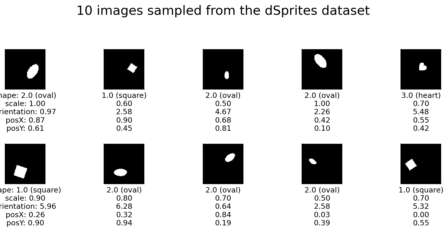
To better understand the posX and posY latent dimensions (which will be most relevant in Bonus 2), we plot the images with some annotations. The annotations (in red) do not modify the actual images; they are added purely for visualization purposes, and show:
the edges of the
posXandposYspans, andthe center, i.e.,
(posX, posY), for each shape.
Note on shape positions: Notice that all shape centers are positioned within the area marked by the red square. posX and posY actually describe the relative position of the center of a shape within this area: posX=0 (left) to posX=1 (right), and posY=0 (top) to posY=1 (bottom). No shape center appears outside, in the buffer area. This choice in the dSprites dataset design ensures that shapes of different scales and rotations all appear fully.
# DEMO: To view different images, set randst to any integer value.
dSprites.show_images(num_images=10, randst=SEED, annotations="pos")
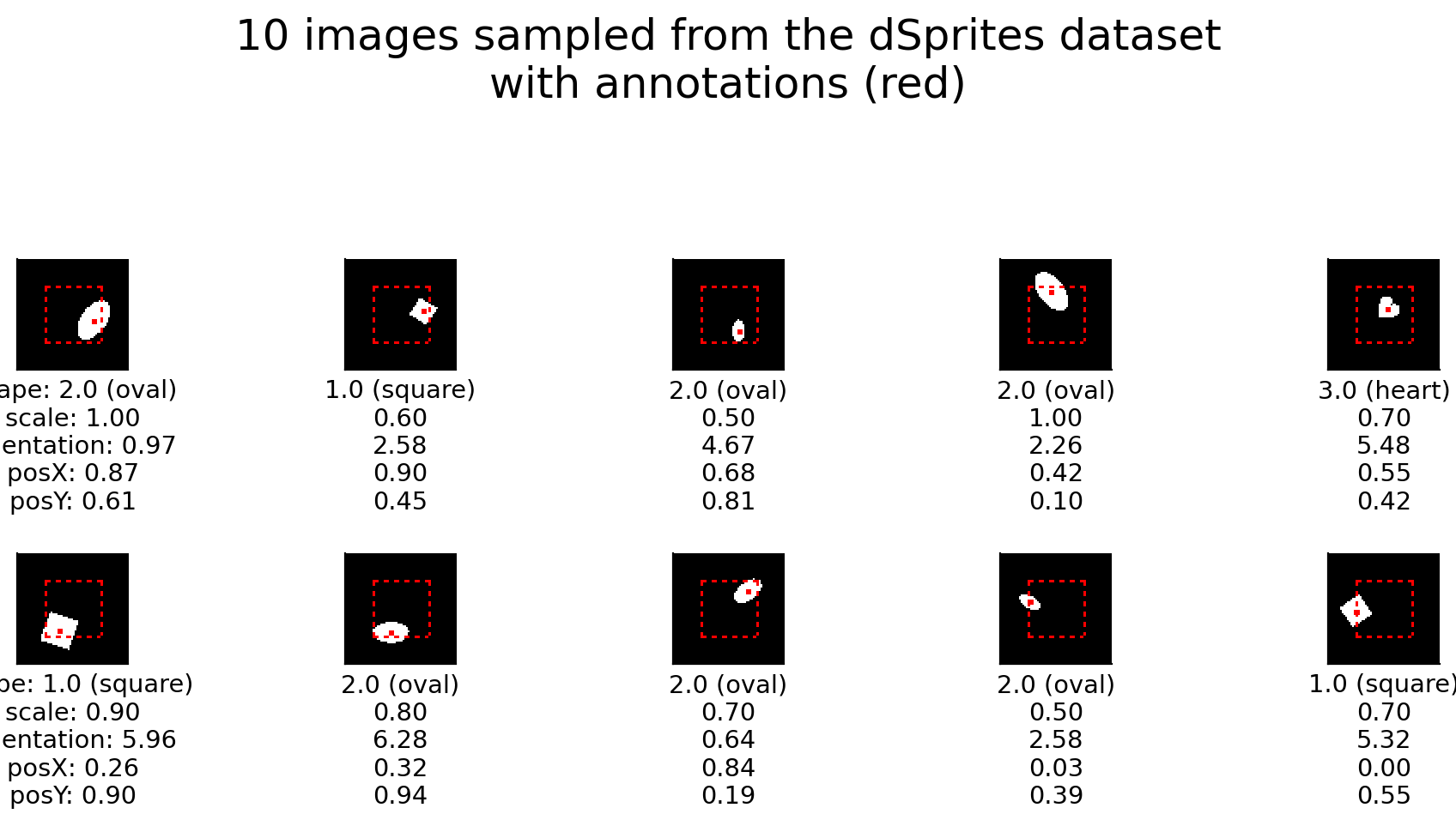
Section 1.2: Training a classifier with and without representations#
Now, we will investigate how 2 different types of classifiers perform when trained to decode the shape latent dimension of images in the dSprites dataset.
Specifically, we will train one classifier directly on the images, and another on the output of an encoder network.
The encoder network we will use here and throughout the tutorial is the multi-layer convolutional network, pictured below. It comprises 2 consecutive convolutional layers, followed by 3 fully connected layers, and uses average pooling and batch normalization between layers, as well as rectified linear units as non-linearities.
The classifier layer then takes the encoder features as input, predicting, for example, the shape latent dimension of encoded input images.
Note on terminology: In this tutorial, both the terms representations and features are used to refer to the data embeddings learned in the final layer of the encoder network (of dimension 1x84, and indicated by a red dashed box) which are fed to the classifiers.
Encoder network schematic#
Show code cell source
# @markdown ### Encoder network schematic
Image(filename=os.path.join(REPO_PATH, "images", "feat_encoder_schematic.png"), width=1200)
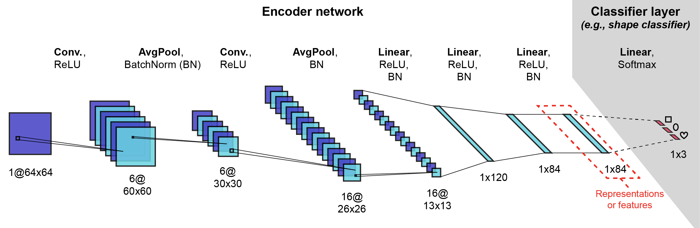
The following code:
Seeds modules that will use random processes, to ensure the results are consistently reproducible, using the
seed_processes()function,Collects the dSprites dataset into a torch dataset using the
data.dSpritesTorchDatasetclass,Initializes a training and a test sampler to keep the two datasets separate using the
data.train_test_splix_idx()function.
# Set the seed before building any dataset/network initializing or training,
# to ensure reproducibility
set_seed(SEED)

# Initialize a torch dataset, specifying the target latent dimension for
# the classifier
dSprites_torchdataset = data.dSpritesTorchDataset(
  dSprites,
  target_latent="shape"
  )

# Initialize a train_sampler and a test_sampler to keep the two sets
# consistently separate
train_sampler, test_sampler = data.train_test_split_idx(
  dSprites_torchdataset,
  fraction_train=0.8,  # 80:20 data split
  randst=SEED
  )

print(f"Dataset size: {len(train_sampler)} training, "
      f"{len(test_sampler)} test images")
Random seed 2021 has been set.
Dataset size: 16000 training, 4000 test images
Interactive Demo 1.2.1: Training a logistic regression classifier directly on images#
The following code:
trains a logistic regression directly on the training set images to classify their shape, and assesses its performance on the test set images using the
models.train_classifier()function.
Interactive Demo: Try a few different num_epochs settings to see whether performance improves with more training, e.g., between 1 and 50 epochs. (The original setting is num_epochs=25).
Submit your feedback#
Show code cell source
# @title Submit your feedback
content_review(f"{feedback_prefix}_What_models_Video")
# Call this before any dataset/network initializing or training,
# to ensure reproducibility
set_seed(SEED)

num_epochs = 25  # DEMO: Try different numbers of training epochs

# Train a classifier directly on the images
print("Training a classifier directly on the images...")
_ = models.train_classifier(
  encoder=None,
  dataset=dSprites_torchdataset,
  train_sampler=train_sampler,
  test_sampler=test_sampler,
  freeze_features=True,  # There is no feature encoder to train here, anyway
  num_epochs=num_epochs,
  verbose=True  # Print results
  )
Random seed 2021 has been set.
Training a classifier directly on the images...
Network performance after 25 classifier training epochs (chance: 33.33%):
    Training accuracy: 51.81%
    Testing accuracy: 39.55%
As we can observe, the classifier trained directly on the images performs only a bit above chance (39.55%) on the test set, after 25 training epochs.
Shape classification results using different feature encoders:
Chance |
None (raw data) |
|
|---|---|---|
33.33% |
39.55% |
Coding Exercise 1.2.1: Training a logistic regression classifier along with an encoder#
The following code:
Uses the same dSprites torch dataset (
dSprites_torchdataset) initialized above, as well as the training and test samplers (train_sampler,test_sampler),Again, seed modules for substructures that use random processes, to ensure the results are consistently reproducible,
Initializes an encoder network to use in the supervised network using the
models.EncoderCoreclass,Sets a proposed number of epochs to use when training the classifier and encoder (
num_epochs=10).
Exercise: Train a classifier, along with the encoder, to classify the input images according to shape, using models.train_classifier(). How does it perform?
Hints:
models.train_classifier():Is introduced in Interactive Demo 1.2.1.
Takes
freeze_featuresas an input argument:If set to
True, the encoder is frozen, and so only the classifier layer is trained.If set to
False, the encoder is not frozen, and is trained along with the classifier layer.
def train_supervised_encoder(num_epochs, seed):
  """
  Helper function to train the encoder in a supervised way

  Args:
    num_epochs: Integer
      Number of epochs the supervised encoder is to be trained for
    seed: Integer
      The seed value for the dataset/network

  Returns:
    supervised_encoder: nn.module
      The trained encoder with mentioned parameters/hyperparameters
  """
  # Call this before any dataset/network initializing or training,
  # to ensure reproducibility
  set_seed(seed)

  # Initialize a core encoder network on which the classifier will be added
  supervised_encoder = models.EncoderCore()

  #################################################
  # Fill in missing code below (...),
  # then remove or comment the line below to test your implementation
  raise NotImplementedError("Exercise: Train a supervised encoder and classifier.")
  #################################################
  # Train an encoder and classifier on the images, using models.train_classifier()
  print("Training a supervised encoder and classifier...")
  _ = models.train_classifier(
      encoder=...,
      dataset=...,
      train_sampler=...,
      test_sampler=...,
      freeze_features=...,
      num_epochs=num_epochs,
      verbose=...  # print results
      )

  return supervised_encoder


num_epochs = 10  # Proposed number of training epochs
## Uncomment below to test your function
# supervised_encoder = train_supervised_encoder(num_epochs=num_epochs, seed=SEED)
Network performance after 10 encoder and classifier training epochs (chance: 33.33%):
    Training accuracy: 100.00%
    Testing accuracy: 98.70%
Submit your feedback#
Show code cell source
# @title Submit your feedback
content_review(f"{feedback_prefix}_Logistic_regression_classifier_Exercise")
When the classifier is trained with an encoder network, however, it achieves very high classification accuracy (~98.70%) on the test set, after only 10 training epochs.
Shape classification results using different feature encoders:
Chance |
None (raw data) |
Supervised |
|
|---|---|---|---|
33.33% |
39.55% |
98.70% |
Section 2: Supervised learning induces invariant representations#
Time estimate: ~20mins
Video 2: Supervised Learning and Invariance#
Submit your feedback#
Show code cell source
# @title Submit your feedback
content_review(f"{feedback_prefix}_Supervised_learning_and_invariance_Video")
Section 2.1: Examining Representational Similarity Matrices (RSMs)#
To examine the representations learned by the encoder network, we use Representational Similarity Matrices (RSMs). In these matrices, the similarity between the encoder’s representations of each possible pair of images is plotted to reveal overall structure in representation space.
Note on cosine similarity: Here, we use cosine similarity as a measure of representational similarity. Cosine similarity measures the angle between 2 vectors, and can be thought of as their normalized dot product.
Coding Exercise 2.1.1: Complete a function that calculates RSMs#
The following code:
Lays out the skeleton of a function
custom_torch_RSM_fct()which calculates an RSM from features,Tests the custom function against the solution implementation.
Exercise: Complete the custom_torch_RSM_fct() implementation.
Hints:
custom_torch_RSM_fct():Takes 1 input argument:
features(2D torch Tensor): Feature matrix (nbr items x nbr features)
Returns 1 output:
rsm(2D torch Tensor): Similarity matrix (nbr items x nbr items)
Uses
torch.nn.functional.cosine_similarity().
torch.nn.functional.cosine_similarity():Takes 3 arguments, in order:
x1(torch Tensor),x2(torch Tensor),dim(int)
Returns the similarity between
x1andx2along dimensiondim.
Detailed hint:
To use
torch.nn.functional.cosine_similarity()to measure the similarity offeaturesto itself for each possible pair of items:Pass 2 versions of
featuresasx1andx2, respectively.Ensure that for
x1andx2, the features dimension is at the same position , and specify that dimension withdim.To obtain the similarity between each possible pair of items, ensure that for
x1andx2, the items dimensions are orthogonal to one another (i.e., at different positions).Don’t forget that to achieve this, singleton dimensions (i.e., dimensions of length 1) can be used.
def custom_torch_RSM_fct(features):
  """
  Custom function to calculate representational similarity matrix (RSM) of a feature
  matrix using pairwise cosine similarity.

  Args:
    features: 2D torch.Tensor
      Feature matrix of size (nbr items x nbr features)

  Returns:
    rsm: 2D torch.Tensor
      Similarity matrix of size (nbr items x nbr items)
  """

  num_items, num_features = features.shape

  #################################################
  # Fill in missing code below (...),
  # Complete the function below given the specific guidelines.
  # Use torch.nn.functional.cosine_similarity()
  # then remove or comment the line below to test your function
  raise NotImplementedError("Exercise: Implement RSM calculation.")
  #################################################
  # EXERCISE: Implement RSM calculation
  rsm = ...

  if not rsm.shape == (num_items, num_items):
    raise ValueError(f"RSM should be of shape ({num_items}, {num_items})")

  return rsm


## Test implementation by comparing output to solution implementation
# test_custom_torch_RSM_fct(custom_torch_RSM_fct)
custom_torch_RSM_fct() is correctly implemented.
Submit your feedback#
Show code cell source
# @title Submit your feedback
content_review(f"{feedback_prefix}_Function_that_calculates_RSMs_Exercise")
Interactive Demo 2.1.1: Plotting the supervised network encoder RSM along different latent dimensions#
In this demo, we calculate an RSM for representations of the test set images generated by the supervised network encoder.
The following code:
Calculates and plots the RSM for the test set, with rows and columns sorted by whichever latent dimension is specified (e.g.,
sorting_latent="shape") usingmodels.plot_model_RSMs().
Interactive Demo: In the current example, the rows and columns of the RSM are organized along the shape latent dimension. Try organizing them along one of the other latent dimensions ("scale", "orientation", "posX" or "posY") to see whether different patterns emerge. (The original setting is sorting_latent="shape".)
sorting_latent = "shape"  # DEMO: Try sorting by different latent dimensions
print("Plotting RSMs...")
_ = models.plot_model_RSMs(
    encoders=[supervised_encoder],  # We pass the trained supervised_encoder
    dataset=dSprites_torchdataset,
    sampler=test_sampler,  # We want to see the representations on the held out test set
    titles=["Supervised network encoder RSM"],  # Plot title
    sorting_latent=sorting_latent,
    )
Plotting RSMs...
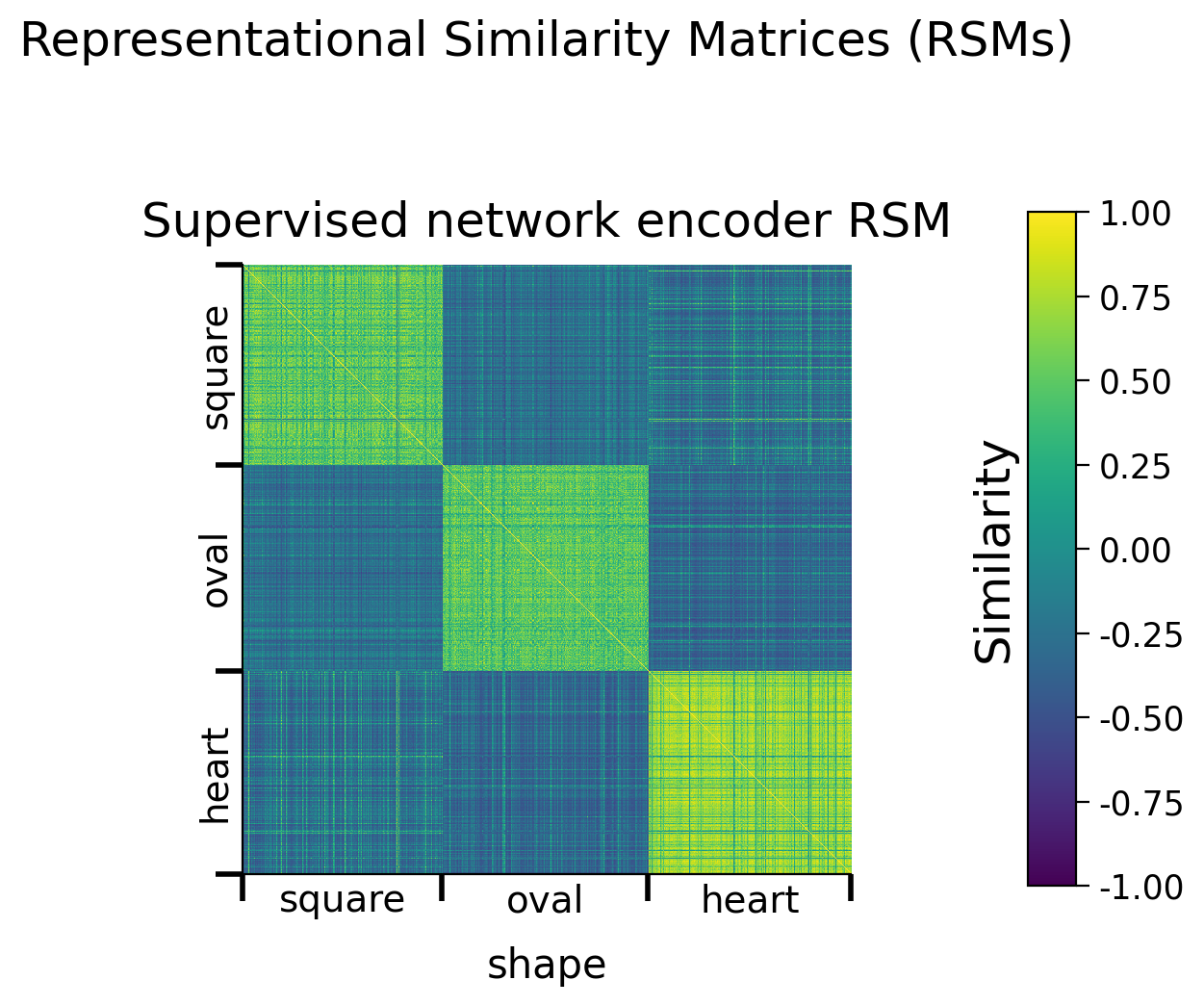
Submit your feedback#
Show code cell source
# @title Submit your feedback
content_review(f"{feedback_prefix}_Supervised_network_encoder_RSM_Interactive_Demo")
Discussion 2.1.1: What patterns do the RSMs reveal about how the encoder represents different images?#
A. What does the yellow (maximal similarity color) diagonal, going from the top left to the bottom right, correspond to? B. What pattern can be observed when comparing RSM values for pairs of images that share a similar latent value (e.g., 2 heart images) vs pairs of images that do not (e.g., a heart and a square image)? C. Do some shapes appear to be encoded more similarly than others? D. Do some latent dimensions show clearer RSM patterns than others? Why might that be so?
Supporting images for Discussion response examples for 2.1.1#
Show code cell source
# @markdown #### Supporting images for Discussion response examples for 2.1.1
Image(filename=os.path.join(REPO_PATH, "images", "rsms_supervised_encoder_10ep_bs1000_seed2021.png"), width=1200)
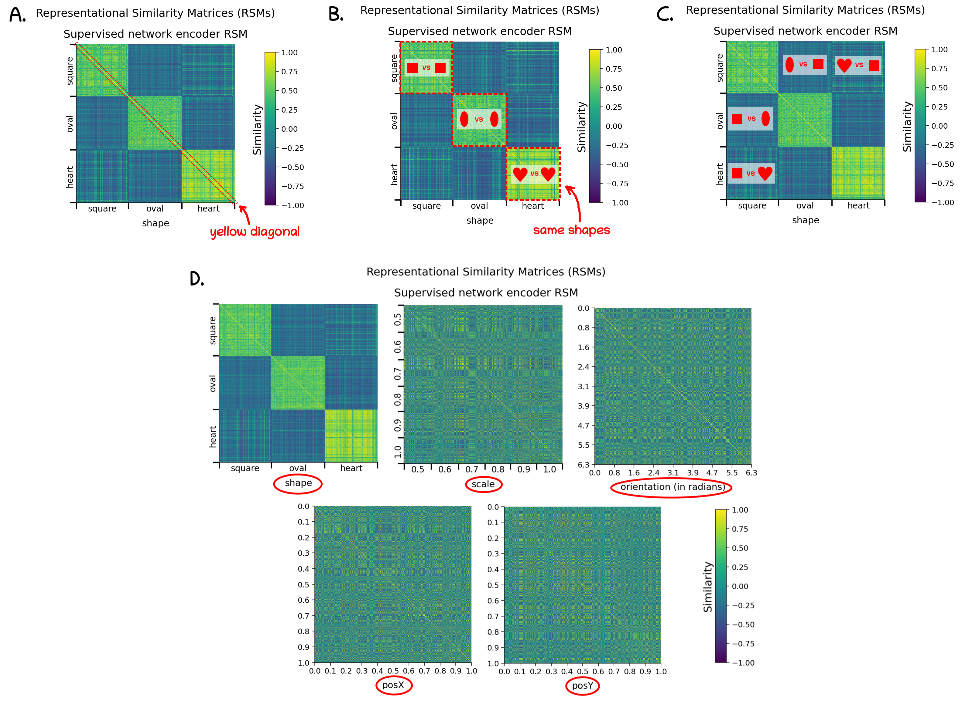
Submit your feedback#
Show code cell source
# @title Submit your feedback
content_review(f"{feedback_prefix}_What_patterns_do_the_RSMs_reveal_Discussion")
Section 3: Random projections don’t work as well#
Time estimate: ~20mins
Video 3: Random Representations#
Submit your feedback#
Show code cell source
# @title Submit your feedback
content_review(f"{feedback_prefix}_Random_representations_Video")
Section 3.1: Examining RSMs of a random encoder#
To determine whether the patterns observed in the RSMs of the supervised network encoder are trivial, we investigate whether they also emerge from the random projections of an untrained encoder.
Coding Exercise 3.1.1: Plotting a random network encoder RSM along different latent dimensions#
In this exercise, we repeat the same analysis as in Section 2.1, but with a random encoder.
The following code:
Initializes an encoder network to use in the random network using the
models.EncoderCoreclass,Proposes a latent dimension along which to sort the rows and columns (
sorting_latent="shape").
Exercise:
Visualize the RSMs for the supervised and random network encoders, using
models.plot_model_RSMs().Visualize the RSMs, organized along different latent dimensions (
"scale","orientation","posX"or"posY"), and compare the patterns observed for the supervised versus the random encoder network.
Hint: models.plot_model_RSMs() is introduced in Interactive Demo 2.1.1.
def plot_rsms(seed):
  """
  Helper function to plot Representational Similarity Matrices (RSMs)

  Args:
    seed: Integer
      The seed value for the dataset/network

  Returns:
    random_encoder: nn.module
      The encoder with mentioned parameters/hyperparameters
  """
  # Call this before any dataset/network initializing or training,
  # to ensure reproducibility
  set_seed(seed)

  # Initialize a core encoder network that will not get trained
  random_encoder = models.EncoderCore()

  # Try sorting by different latent dimensions
  sorting_latent = "shape"

  #################################################
  # Fill in missing code below (...),
  # then remove or comment the line below to test your implementation
  raise NotImplementedError("Exercise: Plot RSMs.")
  #################################################
  # Plot RSMs
  print("Plotting RSMs...")
  _ = models.plot_model_RSMs(
      encoders=[..., ...],  # Pass both encoders
      dataset=...,
      sampler=...,  # To see the representations on the held out test set
      titles=["Supervised network encoder RSM",
              "Random network encoder RSM"],  # Plot titles
      sorting_latent=sorting_latent,
      )

  return random_encoder


## Uncomment below to test your function
# random_encoder = plot_rsms(seed=SEED)
Example output:
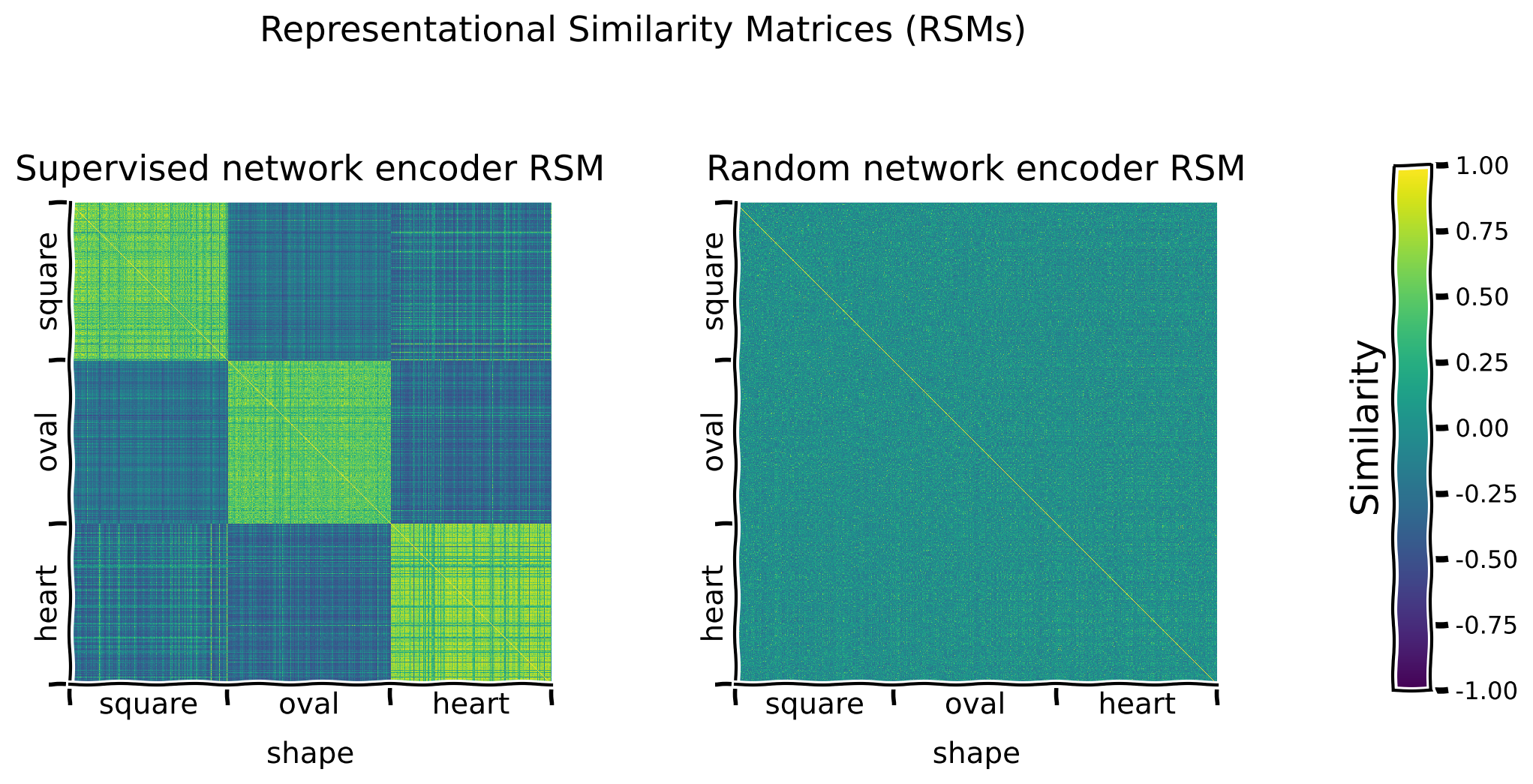
Submit your feedback#
Show code cell source
# @title Submit your feedback
content_review(f"{feedback_prefix}_Plotting_a_random_network_encoder_Exercise")
Discussion 3.1.1: What does comparing these RSMs reveal about the potential value of trained versus random encoder representations?#
A. What patterns, if any, are visible in the random network encoder RSM? B. Which encoder network is most likely to produce meaningful representations?
Supporting images for Discussion response examples for 3.1.1: All random encoder RSMs#
Show code cell source
# @markdown #### Supporting images for Discussion response examples for 3.1.1: All random encoder RSMs
Image(filename=os.path.join(REPO_PATH, "images", "rsms_random_encoder_0ep_bs0_seed2021.png"), width=1000)
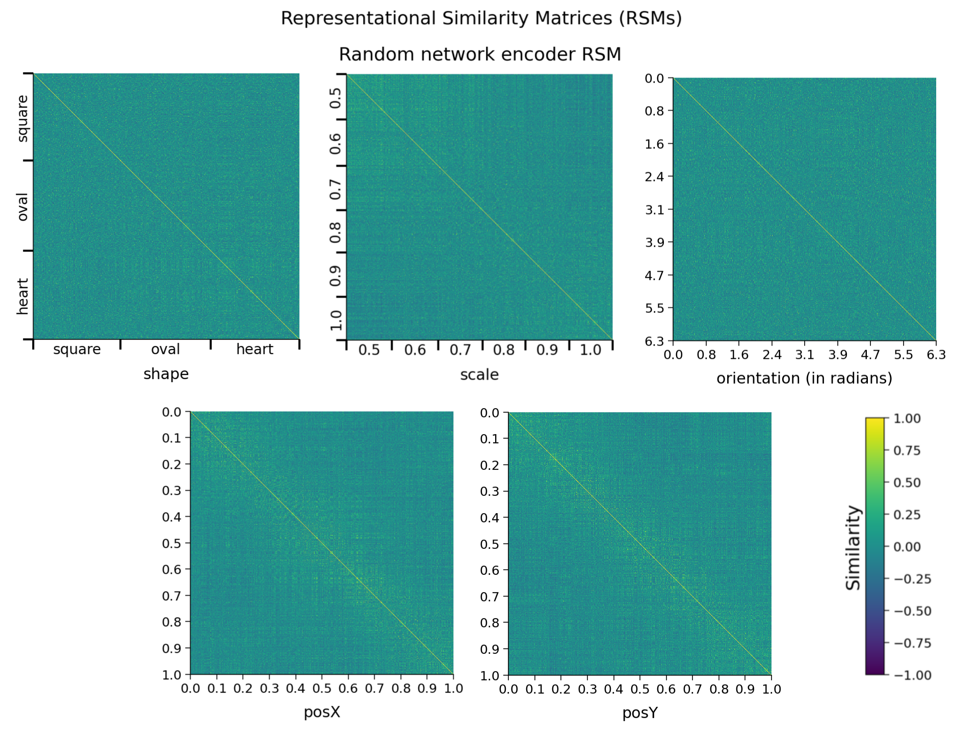
Submit your feedback#
Show code cell source
# @title Submit your feedback
content_review(f"{feedback_prefix}_Trained_vs_Random_encoder_Discussion")
Coding Exercise 3.1.2: Evaluating the classification performance of a logistic regression trained on the representations produced by a random network encoder#
In this exercise, we repeat a similar analysis to Section 1.2, but with the random encoder network. Importantly, this time, the encoder parameters must stay frozen during training by setting freeze_features=True. Instead of being provided ahead of time a suggestion for a reasonable number of training epochs, we use the training loss array to select a good value.
The following code:
Trains a logistic regression on top of the random encoder network to classify images based on shape, and assesses its performance on the test set images using
models.train_classifier()withfreeze_features=Trueto ensure that the encoder is not trained, and only the classifier is.
Exercise:
Set a number of epochs for which to train the classifier.
Plot the training loss array (
random_loss_array, i.e., training loss at each epoch) returned when training the model.Rerun the classifier if more training epochs are needed based on the progression of the training loss.
def plot_loss(num_epochs, seed):
  """
  Helper function to plot the loss function of the random-encoder

  Args:
    num_epochs: Integer
      Number of the epochs the random encoder is to be trained for
    seed: Integer
      The seed value for the dataset/network

  Returns:
    random_loss_array: List
      Loss per epoch
  """
  # Call this before any dataset/network initializing or training,
  # to ensure reproducibility
  set_seed(seed)

  # Train classifier on the randomly encoded images
  print("Training a classifier on the random encoder representations...")
  _, random_loss_array, _, _ = models.train_classifier(
      encoder=random_encoder,
      dataset=dSprites_torchdataset,
      train_sampler=train_sampler,
      test_sampler=test_sampler,
      freeze_features=True,  # Keep the encoder frozen while training the classifier
      num_epochs=num_epochs,
      verbose=True  # Print results
      )
  #################################################
  # Fill in missing code below (...),
  # then remove or comment the line below to test your implementation
  raise NotImplementedError("Exercise: Plot loss array.")
  #################################################
  # Plot the loss array
  fig, ax = plt.subplots()
  ax.plot(...)
  ax.set_title(...)
  ax.set_xlabel(...)
  ax.set_ylabel(...)

  return random_loss_array


## Set a reasonable number of training epochs
num_epochs = 25
## Uncomment below to test your plot
# random_loss_array = plot_loss(num_epochs=num_epochs, seed=SEED)
Network performance after 25 classifier training epochs (chance: 33.33%):
    Training accuracy: 46.02%
    Testing accuracy: 44.67%
Example output:
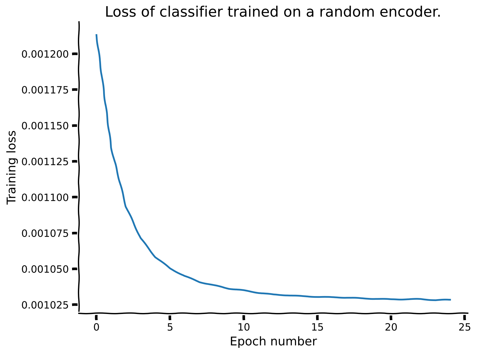
Submit your feedback#
Show code cell source
# @title Submit your feedback
content_review(f"{feedback_prefix}_Evaluating_the_classification_performance_Exercise")
The network loss training is fairly stable by 25 epochs, at which point the classifier performs at 44.67% accuracy on the test dataset.
Shape classification results using different feature encoders:
Chance |
None (raw data) |
Supervised |
Random |
|
|---|---|---|---|---|
33.33% |
39.55% |
98.70% |
44.67% |
Discussion 3.1.2: What can we conclude about the potential consequences of using random projections with a dataset like dSprites?#
A. How does the classifier performance compare to the classifier trained directly on the images? B. How does the classifier performance compare to the classifier trained along with the encoder (supervised encoder)? C. What explains these different performances?
Submit your feedback#
Show code cell source
# @title Submit your feedback
content_review(f"{feedback_prefix}_Random_projections_with_dSprites_Discussion")
Section 4: Generative approaches to representation learning can fail#
Time estimate: ~30mins
Video 4: Generative models#
Submit your feedback#
Show code cell source
# @title Submit your feedback
content_review(f"{feedback_prefix}_Generative_models_Video")
Section 4.1: Examining the RSMs of a Variational Autoencoder#
We next ask - What kind of representations a network can learn in the absence of labelled data? To answer this question, we first look at a generative model, namely the Variational Autoencoder (VAE).
Given that generative models typically require more training than supervised models, instead of pre-training a network here, we will load one that was pre-trained for 300 epochs. Importantly, the encoder shares the same architecture as the one used for the supervised and random examples above.
The following code:
Loads the parameters of a full Variational AutoEncoder (VAE) network (encoder and decoder) pre-trained on the generative task of reconstructing the input images, under the Kullback-Leibler Divergence (KLD) minimization constraint over the latent space that characterizes VAEs, using
load.load_encoder()andload.load_decoder().
# Call this before any dataset/network initializing or training,
# to ensure reproducibility
set_seed(SEED)

# Load VAE encoder and decoder pre-trained on the reconstruction and KLD tasks
vae_encoder = load.load_encoder(REPO_PATH, model_type="vae")
vae_decoder = load.load_vae_decoder(REPO_PATH)
Random seed 2021 has been set.
Loading VAE encoder from 'neuromatch_ssl_tutorial/checkpoints/vae_encoder_300ep_bs500_seed2021.pth'.
    => trained for 300 epochs (batch_size of 500) on the full dSprites subset dataset.
Loading VAE decoder from 'neuromatch_ssl_tutorial/checkpoints/vae_decoder_300ep_bs500_seed2021.pth'.
   => trained for 300 epochs (batch_size of 500) on the full dSprites subset dataset.
Interactive Demo 4.1.1: Plotting example reconstructions using the pre-trained VAE encoder and decoder#
In this demo, we sample images from the test set, and take a look at the quality of the reconstructions using models.plot_vae_reconstructions().
Interactive Demo: Try plotting different images from the test dataset by selecting different test_sampler.indices values. (Original setting is indices=test_sampler.indices[:10].)
models.plot_vae_reconstructions(
    vae_encoder,  # Pre-trained encoder
    vae_decoder,  # Pre-trained decoder
    dataset=dSprites_torchdataset,
    indices=test_sampler.indices[:10],  # DEMO: Select different indices to plot from the test set
    title="VAE test set image reconstructions",
    )
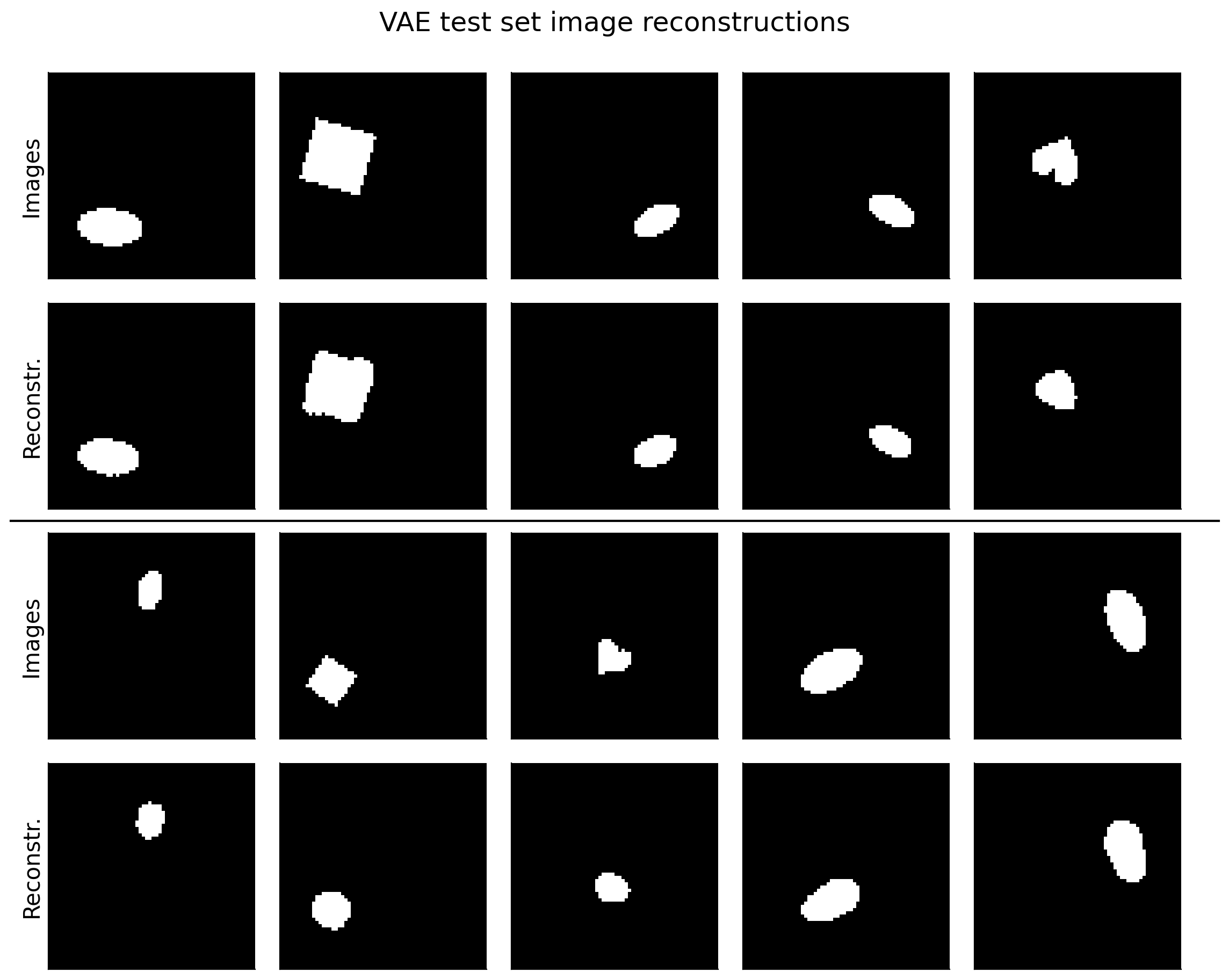
Submit your feedback#
Show code cell source
# @title Submit your feedback
content_review(f"{feedback_prefix}_Pretrained_VAE_Interactive_Demo")
Discussion 4.1.1: How does the VAE perform on the reconstruction task?#
A. Which latent features does the network appear to preserve well, and which does it preserve less well? B. Based on the reconstruction performance, what do you expect to see in the different RSMs?
Note on reconstruction quality: This VAE network uses a basic VAE loss with a convolutional encoder (our core encoder network), and a deconvolutional decoder. This can lead to some blurriness in the reconstructed shapes which a more sophisticated VAE could overcome.
Submit your feedback#
Show code cell source
# @title Submit your feedback
content_review(f"{feedback_prefix}_VAE_on_the_reconstruction_task_Discussion")
Interactive Demo 4.1.2: Visualizing the VAE encoder RSMs, organized along different latent dimensions#
We will now compare the pre-trained VAE encoder network RSM to the previously generated encoder RSMs.
Interactive Demo: Visualize the RSMs, organized along different latent dimensions ("scale", "orientation", "posX" or "posY"), and compare the patterns observed for the different encoder networks. (The original setting is sorting_latent="shape".)
sorting_latent = "shape"  # DEMO: Try sorting by different latent dimensions
print("Plotting RSMs...")
_ = models.plot_model_RSMs(
    encoders=[supervised_encoder, random_encoder, vae_encoder],  # Pass all three encoders
    dataset=dSprites_torchdataset,
    sampler=test_sampler,  # To see the representations on the held out test set
    titles=["Supervised network encoder RSM", "Random network encoder RSM",
            "VAE network encoder RSM"],  # Plot titles
    sorting_latent=sorting_latent,
    )
Plotting RSMs...
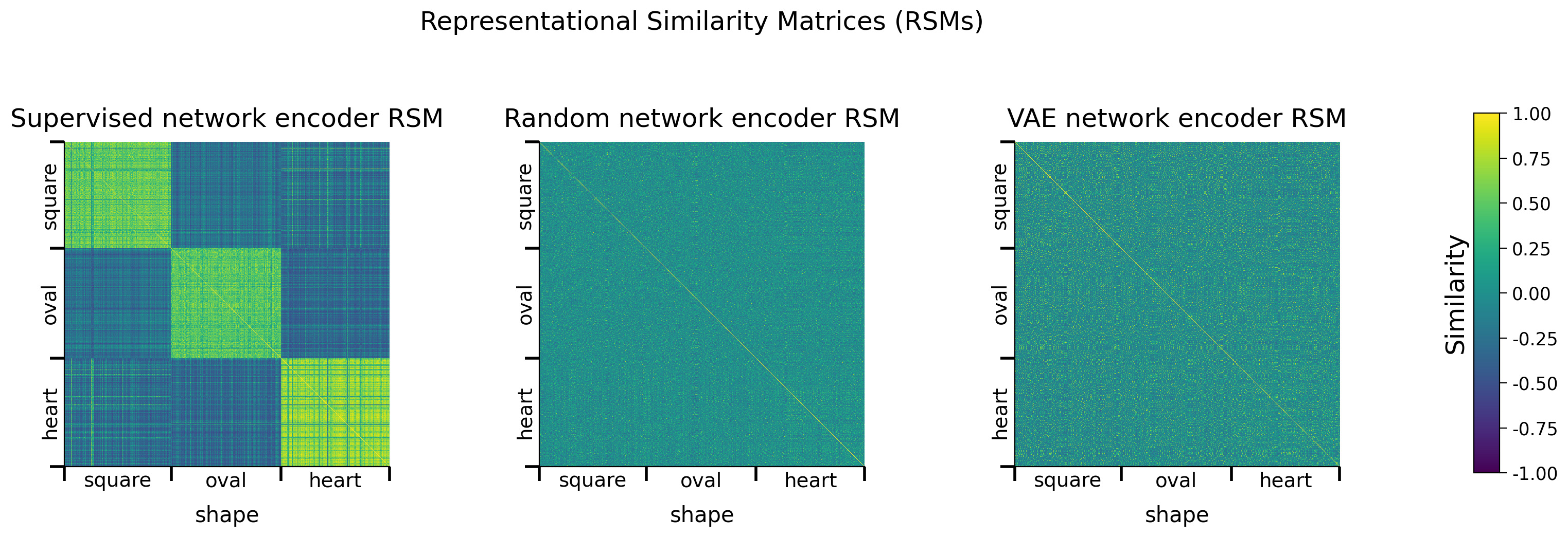
Submit your feedback#
Show code cell source
# @title Submit your feedback
content_review(f"{feedback_prefix}_VAE_encoder_RSMs_Interactive_Demo")
Discussion 4.1.2: What can we conclude about the the ability of generative models like VAEs to construct a meaningful representation space?#
A. What structure can be observed in the pre-trained VAE encoder RSMs when sorted along the different latent dimensions, and what does that suggest about the feature space learned by the VAE encoder? B. How do the pre-trained VAE encoder RSMs compare to the supervised and random encoder network RSMs? C. What explains these different RSMs? D. How well will the pre-trained VAE encoder likely perform on the shape classification task, as compared to the other encoder networks? E. Might the pre-trained VAE encoder be better suited to predicting a different latent dimension?
Supporting images for Discussion response examples for 4.1.2: All VAE encoder RSMs#
Show code cell source
# @markdown #### Supporting images for Discussion response examples for 4.1.2: All VAE encoder RSMs
Image(filename=os.path.join(REPO_PATH, "images", "rsms_vae_encoder_300ep_bs500_seed2021.png"), width=1000)
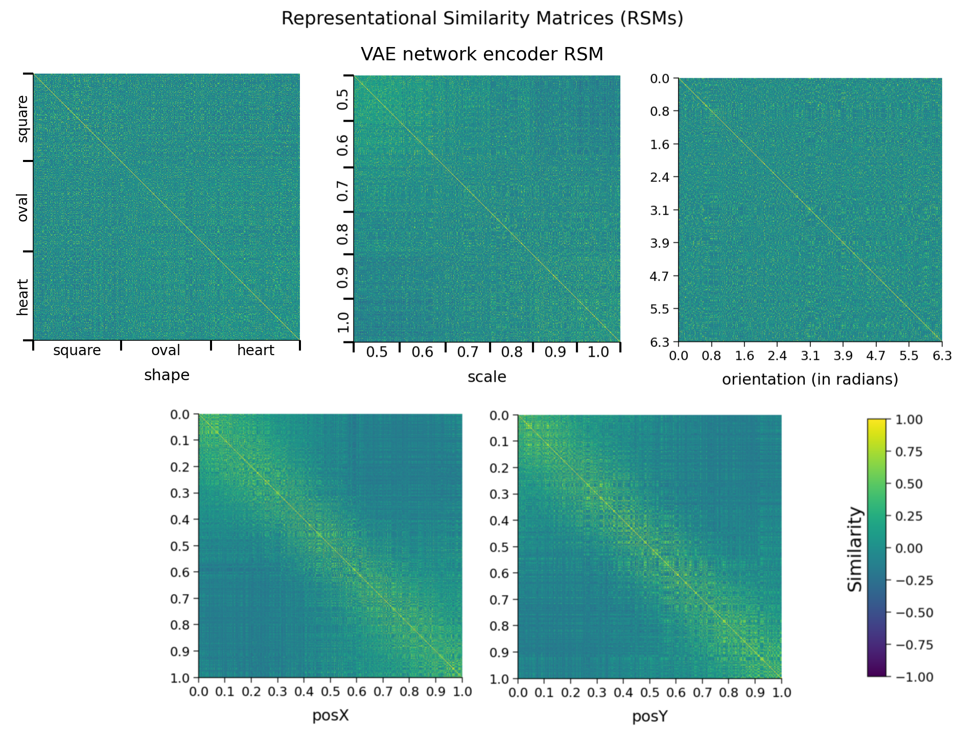
Submit your feedback#
Show code cell source
# @title Submit your feedback
content_review(f"{feedback_prefix}_Construct_a_meaningful_representation_space_Discussion")
Coding Exercise 4.1.2: Evaluating the classification performance of a logistic regression trained on the representations produced by the pre-trained VAE network encoder#
For the pre-trained VAE encoder, as the encoder parameters have already been trained, they should be kept frozen while the classifier is trained by setting freeze_features=True.
Exercise:
Set a number of epochs for which to train the classifier.
Train a classifier, along with the encoder, to classify the input images according to shape, using `models.train_classifier()`.
Plot the loss array returned when training the model, and update the number of training epochs, if needed.
Hint: models.train_classifier() is introduced in Interactive Demo 1.2.1.
def vae_train_loss(num_epochs, seed):
  """
  Helper function to plot the train loss of the variational autoencoder (VAE)

  Args:
    num_epochs: Integer
      Number of the epochs the VAE is to be trained for
    seed: Integer
      The seed value for the dataset/network

  Returns:
    vae_loss_array: List
      Loss per epoch
  """
  # Call this before any dataset/network initializing or training,
  # to ensure reproducibility
  set_seed(seed)
  #################################################
  # Fill in missing code below (...),
  # then remove or comment the line below to test your implementation
  raise NotImplementedError("Exercise: Train a classifer on the pre-trained VAE encoder representations.")
  #################################################
  # Train an encoder and classifier on the images, using models.train_classifier()
  print("Training a classifier on the pre-trained VAE encoder representations...")
  _, vae_loss_array, _, _ = models.train_classifier(
      encoder=...,
      dataset=...,
      train_sampler=...,
      test_sampler=...,
      freeze_features=..., # Keep the encoder frozen while training the classifier
      num_epochs=...,
      verbose=... # Print results
      )
  #################################################
  # Fill in missing code below (...),
  # then remove or comment the line below to test your implementation
  raise NotImplementedError("Exercise: Plot the VAE classifier training loss.")
  #################################################
  # Plot the VAE classifier training loss.
  fig, ax = plt.subplots()
  ax.plot(...)
  ax.set_title(...)
  ax.set_xlabel(...)
  ax.set_ylabel(...)

  return vae_loss_array


# Set a reasonable number of training epochs
num_epochs = 25
## Uncomment below to test your function
# vae_loss_array = vae_train_loss(num_epochs=num_epochs, seed=SEED)
Network performance after 25 classifier training epochs (chance: 33.33%):
    Training accuracy: 46.48%
    Testing accuracy: 45.75%
Example output:
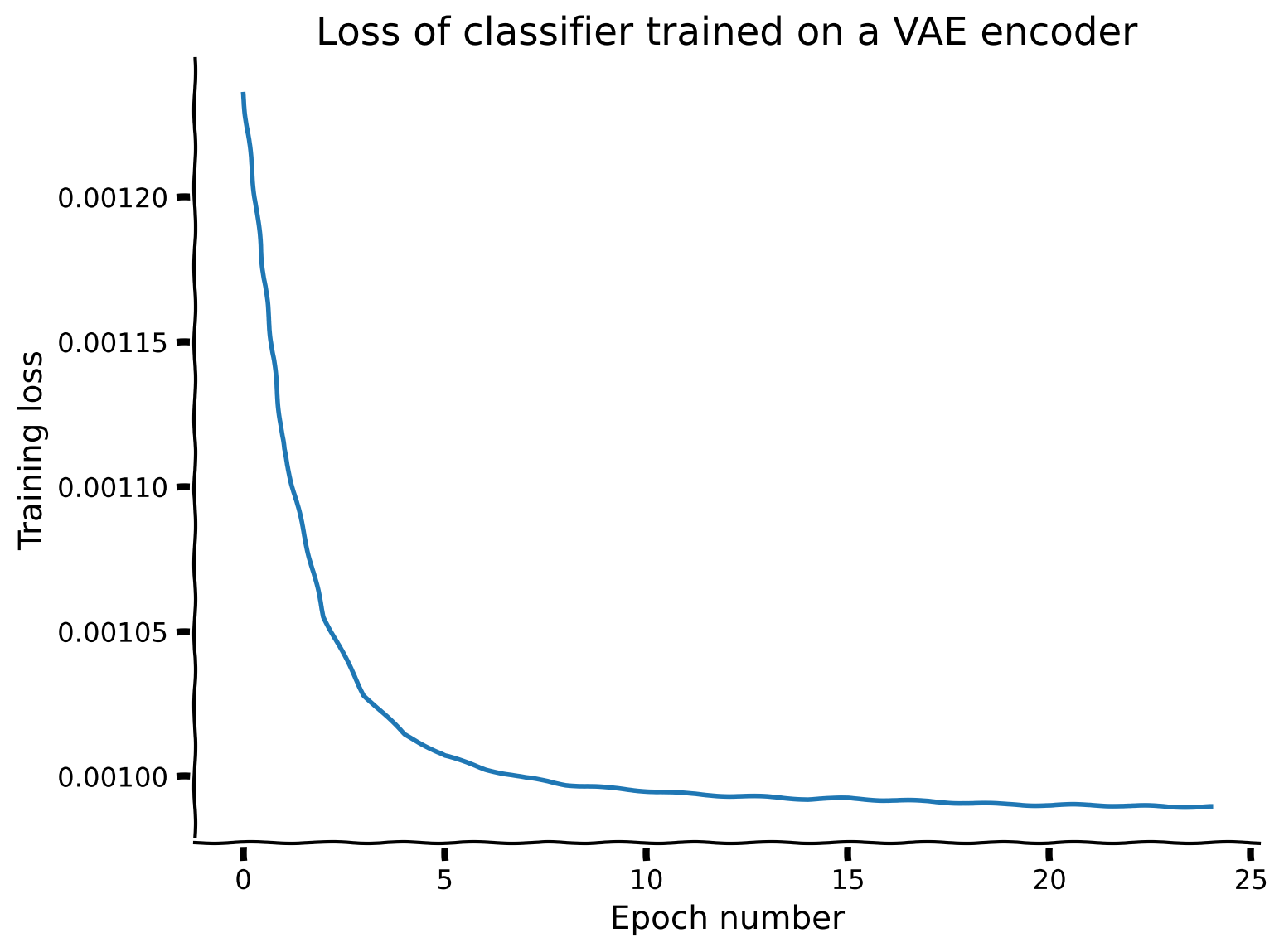
Submit your feedback#
Show code cell source
# @title Submit your feedback
content_review(f"{feedback_prefix}_Evaluate_performance_using_pretrained_VAE_Exercise")
The network loss training is fairly stable by 25 epochs, at which point the classifier performs at 45.75% accuracy on the test dataset.
Shape classification results using different feature encoders:
Chance |
None (raw data) |
Supervised |
Random |
VAE |
|
|---|---|---|---|---|---|
33.33% |
39.55% |
98.70% |
44.67% |
45.75% |
Section 5: The modern approach to self-supervised training for invariance#
Time estimate: ~10mins
Video 5: Modern Approach in Self-supervised Learning#
Submit your feedback#
Show code cell source
# @title Submit your feedback
content_review(f"{feedback_prefix}_Modern_approach_in_Selfsupervised_Learning_Video")
Section 5.1: Examining different options for learning invariant representations.#
We now take a look at a few options for learning invariant shape representations for a dataset such as dSprites.
Interactive Demo 5.1.1: Visualizing a few different image transformations available that could be used to learn invariance#
The following code:
Initializes a set of transforms called
invariance_transformsusing thetorchvision.transforms.RandomAffineclass,Collects the dSprites dataset into a torch dataset
dSprites_invariance_torchdatasetwhich takes theinvariance_transformsas input and deploys the transforms when it is called,Shows a few examples of images and their transformed versions using the
data.dSpritesTorchDatasetshow_images()method.
The torchvision.transforms.RandomAffine class enables us to predetermine which types and ranges of transforms will be sampled from when transforming the images, by setting the following arguments:
degrees: Absolute maximum number of degrees to rotatetranslate: Absolute maximum proportion of width to shift in x, and of height to shift in yscale: Minimum to maximum scaling factor
Interactive Demo: Try out a few combinations of the transformation parameters, and visualize the pairs of transformations of the same image. (The original settings are degrees=90, translate=(0.2, 0.2), scale=(0.8, 1.2).)
# Call this before any dataset/network initializing or training,
# to ensure reproducibility
set_seed(SEED)

# DEMO: Try some random affine data augmentations combinations to apply to the images
invariance_transforms = torchvision.transforms.RandomAffine(
    degrees=90,
    translate=(0.2, 0.2),  # (in x, in y)
    scale=(0.8, 1.2)   # min to max scaling
    )

# Initialize a simclr-specific torch dataset
dSprites_invariance_torchdataset = data.dSpritesTorchDataset(
    dSprites,
    target_latent="shape",
    simclr=True,
    simclr_transforms=invariance_transforms
    )

# Show a few example of pairs of image augmentations
_ = dSprites_invariance_torchdataset.show_images(randst=SEED)
Random seed 2021 has been set.
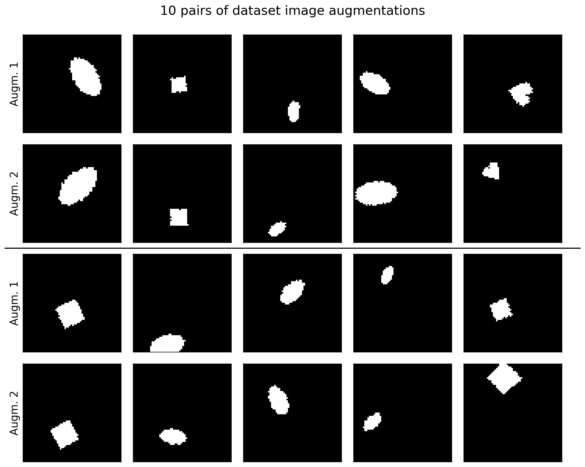
Submit your feedback#
Show code cell source
# @title Submit your feedback
content_review(f"{feedback_prefix}_Image_transformations_Interactive_Demo")
Section 6: How to train for invariance to transformations with a target network#
Time estimate: ~40mins
Video 6: Data Transformations#
Submit your feedback#
Show code cell source
# @title Submit your feedback
content_review(f"{feedback_prefix}_Data_Transformations_Video")
Section 6.1: Using image transformations to learn feature invariant representations in a Self-supervised Learning (SSL) network.#
We will now investigate the effects of selecting certain transformations compared to others on the invariance learned by an encoder network trained with a specific type of SSL algorithm, namely SimCLR. Specifically, we will observe how pre-training an encoder network with SimCLR affects the performance of a classifier trained on the representations the network has learned.
Coding Exercise 6.1.1: Complete a SimCLR loss function#
The following code:
Lays out the skeleton of a function
custom_simclr_contrastive_loss()which calculates the contrastive loss for a SimCLR network,Tests the custom function against the solution implementation,
Trains SimCLR for a few epochs.
Exercise:
Complete the
custom_simclr_contrastive_loss()implementation,Plot the loss after training SimCLR with the custom loss function for a few epochs.
Detailed hint:
custom_simclr_contrastive_loss():Takes 2 input arguments:
proj_feat1(2D torch Tensor): Projected features for first image augmentations (batch_size x feat_size)proj_feat2(2D torch Tensor): Projected features for second image augmentations (batch_size x feat_size)
Computes the
similarity_matrixfor all possible pairs of image augmentations.Identifies positive and negative sample indicators for indexing the
similarity_matrix:pos_sample_indicators(2D torch Tensor): Tensor indicating the positions of positive image pairs with 1s (and 0s in all other positions). (batch_size * 2 x batch_size * 2)neg_sample_indicators(2D torch Tensor): Tensor indicating the positions of negative image pairs with 1s (and 0s in all other positions). (batch_size * 2 x batch_size * 2)
Computes the 2 parts of the contrastive loss, retrieving the relevant values from the
similarity_matrixusing the indicators:numerator: Calculated from thesimilarity_matrixvalues for positive pairs.denominator: Calculated from thesimilarity_matrixvalues for negative pairs.
def custom_simclr_contrastive_loss(proj_feat1, proj_feat2, temperature=0.5):
  """
  Returns contrastive loss, given sets of projected features, with positive
  pairs matched along the batch dimension.

  Args:
    Required:
      proj_feat1: 2D torch.Tensor
        Projected features for first image with augmentations (size: batch_size x feat_size)
      proj_feat2: 2D torch.Tensor
        Projected features for second image with augmentations (size: batch_size x feat_size)
    Optional:
      temperature: Float
        relaxation temperature (default: 0.5)
        l2 normalization along with temperature effectively weights different
        examples, and an appropriate temperature can help the model learn from hard negatives.
  Returns:
    loss: Float
      Mean contrastive loss
  """
  device = proj_feat1.device

  if len(proj_feat1) != len(proj_feat2):
    raise ValueError(f"Batch dimension of proj_feat1 ({len(proj_feat1)}) "
                     f"and proj_feat2 ({len(proj_feat2)}) should be same")

  batch_size = len(proj_feat1) # N
  z1 = torch.nn.functional.normalize(proj_feat1, dim=1)
  z2 = torch.nn.functional.normalize(proj_feat2, dim=1)

  proj_features = torch.cat([z1, z2], dim=0) # 2N x projected feature dimension
  similarity_matrix = torch.nn.functional.cosine_similarity(
      proj_features.unsqueeze(1), proj_features.unsqueeze(0), dim=2
      ) # dim: 2N x 2N

  # Initialize arrays to identify sets of positive and negative examples, of
  # shape (batch_size * 2, batch_size * 2), and where
  # 0 indicates that 2 images are NOT a pair (either positive or negative, depending on the indicator type)
  # 1 indices that 2 images ARE a pair (either positive or negative, depending on the indicator type)
  pos_sample_indicators = torch.roll(torch.eye(2 * batch_size), batch_size, 1).to(device)
  neg_sample_indicators = (torch.ones(2 * batch_size) - torch.eye(2 * batch_size)).to(device)

  #################################################
  # Fill in missing code below (...),
  # then remove or comment the line below to test your function
  raise NotImplementedError("Exercise: Implement SimCLR loss.")
  #################################################
  # Implement the SimClr loss calculation
  # Calculate the numerator of the Loss expression by selecting the appropriate elements from similarity_matrix.
  # Use the pos_sample_indicators tensor
  numerator = ...

  # Calculate the denominator of the Loss expression by selecting the appropriate elements from similarity_matrix,
  # and summing over pairs for each item.
  # Use the neg_sample_indicators tensor
  denominator = ...

  if (denominator < 1e-8).any(): # Clamp to avoid division by 0
    denominator = torch.clamp(denominator, 1e-8)

  loss = torch.mean(-torch.log(numerator / denominator))

  return loss


## Uncomment below to test your function
# test_custom_contrastive_loss_fct(custom_simclr_contrastive_loss)
custom_simclr_contrastive_loss() is correctly implemented.
Submit your feedback#
Show code cell source
# @title Submit your feedback
content_review(f"{feedback_prefix}_SimCLR_loss_function_Exercise")
We can now train the SimCLR encoder with the custom contrastive loss for a few epochs.
# Call this before any dataset/network initializing or training,
# to ensure reproducibility
set_seed(SEED)

# Train SimCLR for a few epochs
print("Training a SimCLR encoder with the custom contrastive loss...")
num_epochs = 5
_, test_simclr_loss_array = models.train_simclr(
    encoder=models.EncoderCore(),
    dataset=dSprites_invariance_torchdataset,
    train_sampler=train_sampler,
    num_epochs=num_epochs,
    loss_fct=custom_simclr_contrastive_loss
    )

# Plot SimCLR loss over a few epochs.
fig, ax = plt.subplots()
ax.plot(test_simclr_loss_array)
ax.set_title("SimCLR network loss")
ax.set_xlabel("Epoch number")
_ = ax.set_ylabel("Training loss")
Given that self-supervised models typically require more training than supervised models, instead of fully pre-training a network here, we will load one that was pre-trained for 60 epochs. Again, the encoder shares the same architecture as the one used for the supervised, random and VAE examples above.
The following code:
Loads the parameters of a SimCLR network pre-trained on the SimCLR contrastive task using
load.load_encoder().
# Load SimCLR encoder pre-trained on the contrastive loss
simclr_encoder = load.load_encoder(REPO_PATH, model_type="simclr")
Loading SimCLR encoder from 'neuromatch_ssl_tutorial/checkpoints/simclr_encoder_60ep_bs1000_deg90_trans0-2_scale0-8to1-2_seed2021.pth'.
    => trained for 60 epochs (batch_size of 1000) on the full dSprites subset dataset
with the following random affine transforms:
	degrees=90
	translation=(0.2, 0.2)
	scale=(0.8, 1.2).
Interactive Demo 6.1.1: Evaluating the classification performance of a logistic regression trained on the representations produced by a SimCLR network encoder that was pre-trained using different image transformations#
For the pre-trained SimCLR encoder, as with the VAE encoder, as the encoder parameters have already been trained, they should be kept frozen while the classifier is trained by setting freeze_features=True.
We train and test with dSprites_torch dataset instead of dSprites_invariance_torch dataset, as we are interested in the classifier performance on the real dSprites images, and not their augmentations.
Interactive Demo: Try different numbers of epochs for which to train the classifier. (The original setting is num_epochs=10.)
# Call this before any dataset/network initializing or training,
# to ensure reproducibility
set_seed(SEED)

print("Training a classifier on the pre-trained SimCLR encoder representations...")
_, simclr_loss_array, _, _ = models.train_classifier(
    encoder=simclr_encoder,
    dataset=dSprites_torchdataset,
    train_sampler=train_sampler,
    test_sampler=test_sampler,
    freeze_features=True,  # Keep the encoder frozen while training the classifier
    num_epochs=10,  # DEMO: Try different numbers of epochs
    verbose=True
    )

fig, ax = plt.subplots()
ax.plot(simclr_loss_array)
ax.set_title("Loss of classifier trained on a SimCLR encoder.")
ax.set_xlabel("Epoch number")
_ = ax.set_ylabel("Training loss")
Random seed 2021 has been set.
Training a classifier on the pre-trained SimCLR encoder representations...
Network performance after 10 classifier training epochs (chance: 33.33%):
    Training accuracy: 97.83%
    Testing accuracy: 97.53%
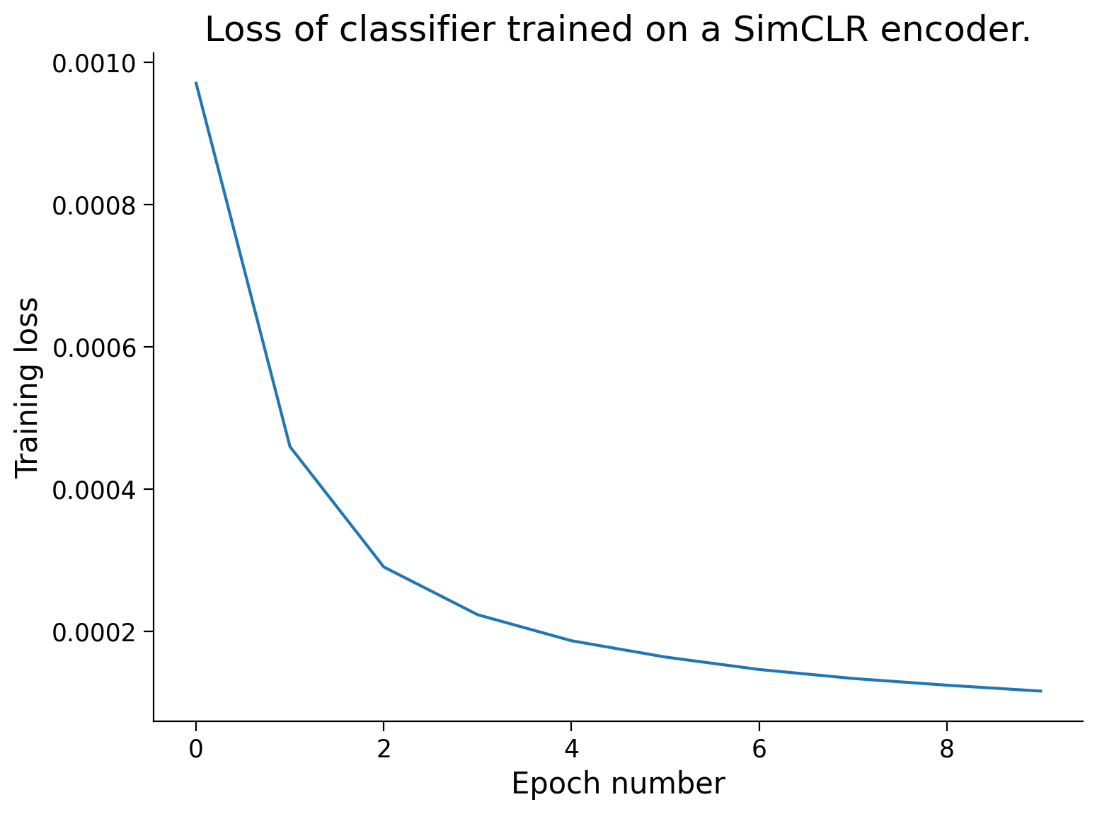
Network performance after 10 classifier training epochs (chance: 33.33%):
    Training accuracy: 97.83%
    Testing accuracy: 97.53%
Submit your feedback#
Show code cell source
# @title Submit your feedback
content_review(f"{feedback_prefix}_Evaluate_performance_using_pretrained_SimCLR_Interactive_Demo")
The network (using the transforms proposed above) performs at 97.53% accuracy on the test dataset, after 15 classifier training epochs.
Shape classification results using different feature encoders:
Chance |
None (raw data) |
Supervised |
Random |
VAE |
SimCLR |
|
|---|---|---|---|---|---|---|
33.33% |
39.55% |
98.70% |
44.67% |
45.75% |
97.53% |
Section 7: Ethical considerations for self-supervised learning from biased datasets#
Video 7: Un/Self-Supervised Learning#
Submit your feedback#
Show code cell source
# @title Submit your feedback
content_review(f"{feedback_prefix}_Un_self_supervised_learning_Video")
Section 7.1: The consequences of training models on biased datasets#
If a model is trained on a biased dataset, it is likely to learn a representational encoding that reproduces these biases, impairing its ability to generalize properly and increasing the likelihood that it will propagate these biases forward.
Here, we investigate the effects of training the models on a biased subset of the training dataset. Specifically, we introduce a train_sampler_biased, a training dataset sampler that only samples:
Squares, if they are centered on the lefthand side of an image (posX: 0 to 0.3),
Ovals, if they are centered in the center of an image (posX: 0.35 to 0.65),
Hearts, if they are centered on the righthand side of am image (posX: 0.7 to 1.0).
This sampling bias introduces a correlation between shape and posX that does not exist in the original dataset.
We then train each model as above on the dataset, and observe their performance when tested on an unbiased dataset.
Note on dataset size: This biased sampling also significantly reduces the size of the training dataset available (approximately 6x). Thus, it would not be fair to compare our results here to those obtained previously in the tutorial, when we were using the full dataset. For this reason, as a control, we will also separately train the models with train_sampler_bias_ctrl, a training dataset sampler that does not share the same sampling bias as train_sampler_biased, but can only sample as many samples as train_sampler_biased can.
# Call this before any dataset/network initializing or training,
# to ensure reproducibility
set_seed(SEED)

bias_type = "shape_posX_spaced"  # Name of bias

# Initialize a biased training sampler and an unbiased test sampler
train_sampler_biased, test_sampler_for_biased = data.train_test_split_idx(
    dSprites_torchdataset,
    fraction_train=0.95,  # 95:5 Split to partially compensate for loss of training examples due to bias
    randst=SEED,
    train_bias=bias_type
    )

# Initialize a control, unbiased training sampler and an unbiased test sampler
train_sampler_bias_ctrl, test_sampler_for_bias_ctrl = data.train_test_split_idx(
    dSprites_torchdataset,
    fraction_train=0.95,
    randst=SEED,
    train_bias=bias_type,
    control=True
    )

print(f"Biased dataset: {len(train_sampler_biased)} training, "
      f"{len(test_sampler_for_biased)} test images")
print(f"Bias control dataset: {len(train_sampler_bias_ctrl)} training, "
      f"{len(test_sampler_for_bias_ctrl)} test images")
Random seed 2021 has been set.
Biased dataset: 5808 training, 1000 test images
Bias control dataset: 5808 training, 1000 test images
We plot some images sampled with train_sampler_biased to observe the pattern described above where shape and posX are now correlated.
To better visualize the bias introduced, we will plot them with annotations that show, in red:
The edges of each of the 3
posXsections, andThe center, i.e.
(posX, posY), for each shape.
print("Plotting first 20 images from the biased training dataset.\n")
dSprites.show_images(indices=train_sampler_biased.indices[:20], annotations="posX_quadrants")
Plotting first 20 images from the biased training dataset.
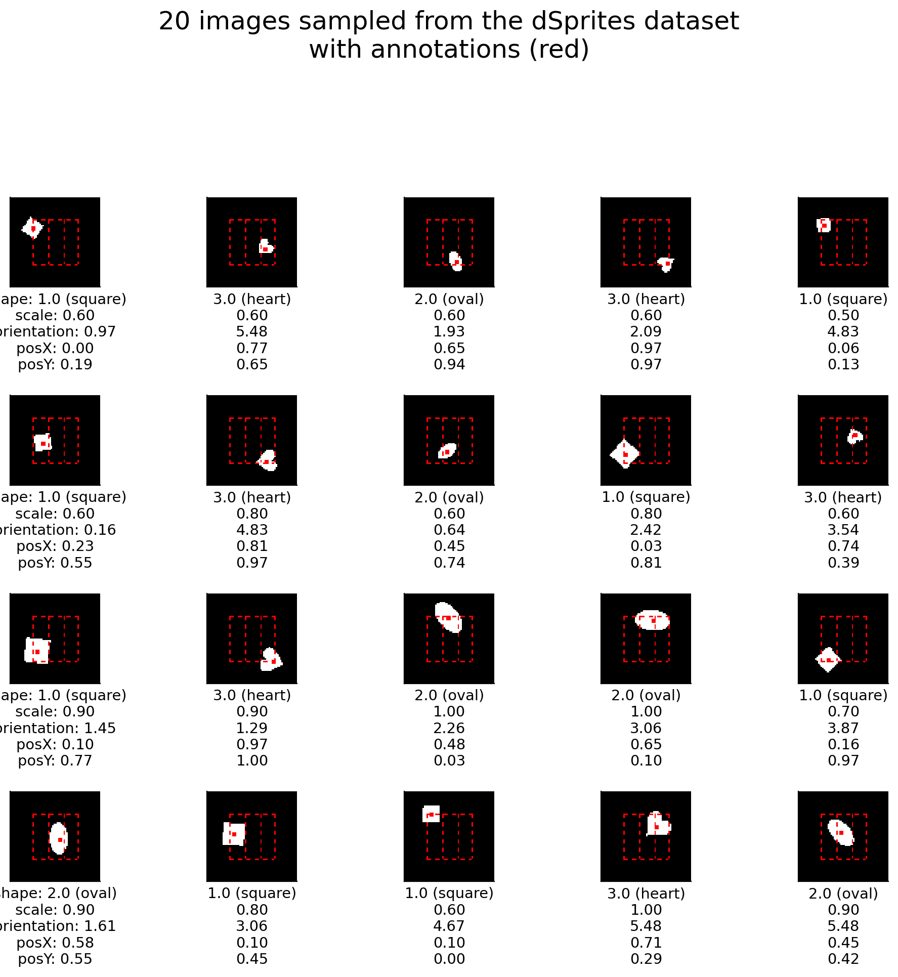
We also plot some images sampled with train_sampler_bias_ctrl to verify visually that this biased pattern does not appear in the control dataset.
Again, the annotations are added, purely for visualization purposes.
print("Plotting sample images from the bias control training dataset.\n")
dSprites.show_images(indices=train_sampler_bias_ctrl.indices[:20], annotations="posX_quadrants")
Plotting sample images from the bias control training dataset.
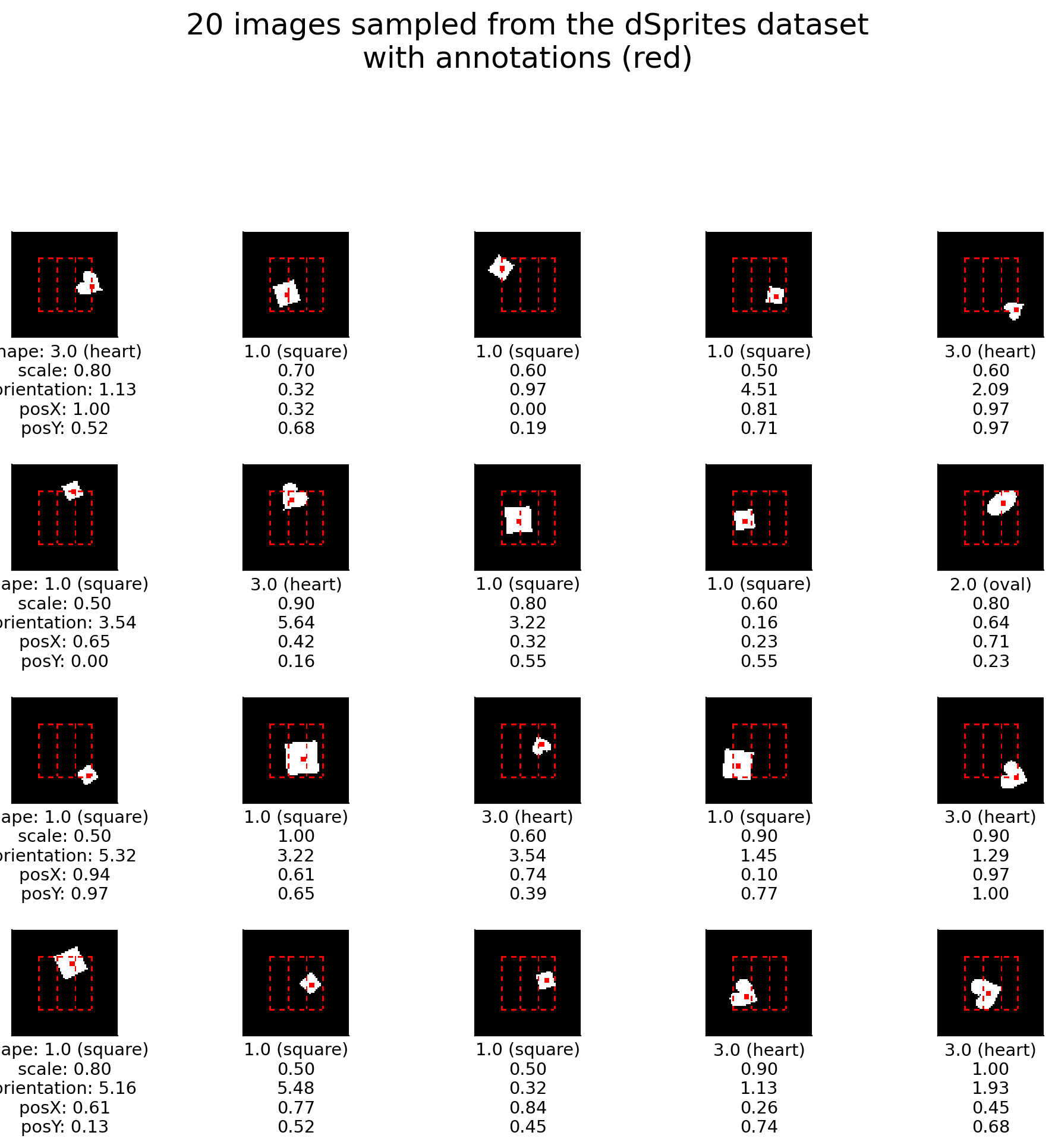
Show code cell source
# @markdown ### Function to run full training procedure
# @markdown (from initializing and pretraining encoders to training classifiers):

# @markdown `full_training_procedure(train_sampler, test_sampler)`

def full_training_procedure(train_sampler, test_sampler, title=None,
                            dataset_type="biased", verbose=True):
  """
  Funtion to load pretrained VAE and SimCLR encoders

  Args:
    train_sampler: torch.Tensor
      Training Data
    test_sampler: torch.Tensor
      Test Data
    title: String
      Title
    dataset_type: String
      Specifies if the expected model type is biased/bias-controlled
    verbose: Boolean
      If true, the shell shows all lines in the script in execution

  Returns:
    Nothing
  """
  if dataset_type not in ["biased", "bias_ctrl"]:
    raise ValueError("Expected model_type to be 'biased' or 'bias_ctrl', "
                     f"but found {model_type}.")

  supervised_encoder = models.EncoderCore()
  random_encoder = models.EncoderCore()

  # Load pre-trained VAE
  vae_encoder = load.load_encoder(
      REPO_PATH, model_type="vae", dataset_type=dataset_type,
      verbose=verbose
      )

  # Load pre-trained SimCLR encoder
  simclr_encoder = load.load_encoder(
      REPO_PATH, model_type="simclr", dataset_type=dataset_type,
      verbose=verbose
      )

  encoders = [supervised_encoder, random_encoder, vae_encoder, simclr_encoder]
  freeze_features = [False, True, True, True]
  encoder_labels = ["supervised", "random", "VAE", "SimCLR"]

  num_clf_epochs = [80, 30, 30, 30]
  print(f"\nTraining supervised encoder and classifier for {num_clf_epochs[0]} "
    f"epochs, and all other classifiers for {num_clf_epochs[1]} epochs each.")
  _ = models.train_encoder_clfs_by_fraction_labelled(
      encoders=encoders,
      dataset=dSprites_torchdataset,
      train_sampler=train_sampler,
      test_sampler=test_sampler,
      num_epochs=num_clf_epochs,
      freeze_features=freeze_features,
      subset_seed=SEED,
      encoder_labels=encoder_labels,
      title=title,
      verbose=verbose
      )
Here, we use a biased training data sampler (and unbiased control sampler) to observe how the different models perform. Because the dataset is much smaller, we increase the number of pre-trained and training epochs for the encoders and classifiers.
Let us start with our unbiased control sampler, to get a sense of the classification performance levels we should expect with a dataset this size.
# Call this before any dataset/network initializing or training,
# to ensure reproducibility
if DEVICE != "cpu":
    set_seed(SEED)

    print("Training all models using the control, unbiased training dataset\n")
    full_training_procedure(
        train_sampler_bias_ctrl, test_sampler_for_bias_ctrl,
        title="Classifier performances with control, unbiased training dataset",
        dataset_type="bias_ctrl"  # For loading correct pre-trained networks
        )
A similar pattern is observed here as with the full dataset, though notably most performances are a bit weaker, likely due to us (A) using a smaller training dataset, and (B) training and pre-training for fewer iterations, considering the dataset size, for time-efficiency reasons.
Using the same parameters, we now repeat the analysis with the biased training data sampler.
# Call this before any dataset/network initializing or training,
# to ensure reproducibility
if DEVICE != "cpu":
    set_seed(SEED)

    print("Training all models using the biased training dataset\n")
    full_training_procedure(
        train_sampler_biased, test_sampler_for_biased,
        title="Classifier performances with biased training dataset",
        dataset_type="biased"  # For loading correct pre-trained networks
        )
Interestingly, the SimCLR network encoder is not only the only network to perform well, it even outperforms its control performance (which uses the same test dataset), at least with this particular dataset and biasing.
Note on performance improvement: This improvement for the SimCLR encoder is reflected in the pre-training loss curves (not shown here), which show that the encoder trained with the biased dataset learns faster than the encoder trained with the unbiased training set. It is possible that the dataset biasing, by reducing the variability in the dataset, makes the contrastive task easier, thus enabling the network to learn a good feature space for the classification task in fewer epochs
Discussion 7.1.1: How do different models cope with a biased training dataset?#
A. Which models are most and least affected by the biased training dataset? B. Which types of images in the test set are most likely causing the observed drop in performance? C. Why are certain models more robust to the bias introduced here than others? D. What are some methods we can employ to help mitigate the negative effects of biases in our training sets on our ability to learn good data representations with our models?
Submit your feedback#
Show code cell source
# @title Submit your feedback
content_review(f"{feedback_prefix}_Biased_training_dataset_Discussion")
Discussion 7.1.2: How do these principles apply more generally?#
We have seen now how self-supervised learning (SSL) can improve a network’s ability to learn good representations of data. For the purposes of this tutorial, we presented examples with a simplified dataset: the dSprites dataset, where we know: (1) The latent dimensions for all images, (2) The joint probability distribution across latent dimensions for the full dataset, and (3) The precise nature of the bias introduced into our biased dataset (see Bonus 2 for more details).
As a result, it is quite simple to design data augmentations that ensure that the pre-trained encoder will learn a good feature space for the downstream classification task.
In real-world applications, with more complex or difficult datasets,
A. What principles can we draw on to successfully apply SSL to learn good data representations in feature space? For example,
B. What challenges might we face with new datasets, compared to applying SSL to dSprites?
C. What types of augmentations might we use when working with non visual datasets, e.g., a speech dataset. In addition, we primarily discussed only one type of SSL, namely SimCLR. However, many different types of SSL exist, some of which do not use explicit data augmentations.
D. What type of SSL task could be implemented for sequential or time series data. For example, you might wish to predict from electrical brain recordings what stage of sleep a person is in. How might you use the knowledge that sleep stages change slowly in time to construct a useful SSL task?
Submit your feedback#
Show code cell source
# @title Submit your feedback
content_review(f"{feedback_prefix}_General_Principles_Discussion")
Summary#
Video 8: Conclusion#
Submit your feedback#
Show code cell source
# @title Submit your feedback
content_review(f"{feedback_prefix}_Conclusion_Video")
Bonus 1: Self-supervised networks learn representation invariance#
Time estimate: ~20mins
Video 9: Invariant Representations#
Submit your feedback#
Show code cell source
# @title Submit your feedback
content_review(f"{feedback_prefix}_Invariant_Representations_Bonus_Video")
Bonus 1.1: The effects of using data transformations on invariance in SimCLR network representations#
We now observe the effects of adding our data transformations on the invariance learned by a pre-trained SimCLR network encoder.
Bonus Interactive Demo 1.1.1: Visualizing the SimCLR network encoder RSMs, organized along different latent dimensions#
We will now compare the pre-trained SimCLR encoder network RSM to the previously generated encoder RSMs.
Again, we pass dSprites_torchdataset instead of dSprites_invariance_torchdataset, as we are interested in the RSMs for the real dSprites images, and not their augmentations.
Interactive Demo: Visualize the RSMs, organized along different latent dimensions ("scale", "orientation", "posX" or "posY"), and compare the patterns observed for the different encoder networks. (The original setting is sorting_latent="shape".)
sorting_latent = "shape"  # DEMO: Try sorting by different latent dimensions
print("Plotting RSMs...")
_ = models.plot_model_RSMs(
    encoders=[supervised_encoder, vae_encoder, simclr_encoder],
    dataset=dSprites_torchdataset,
    sampler=test_sampler,  # To see the representations on the held out test set
    titles=["Supervised network encoder RSM", "VAE network encoder RSM",
            "SimCLR network encoder RSM"],  # Plot titles
    sorting_latent=sorting_latent
    )
Plotting RSMs...
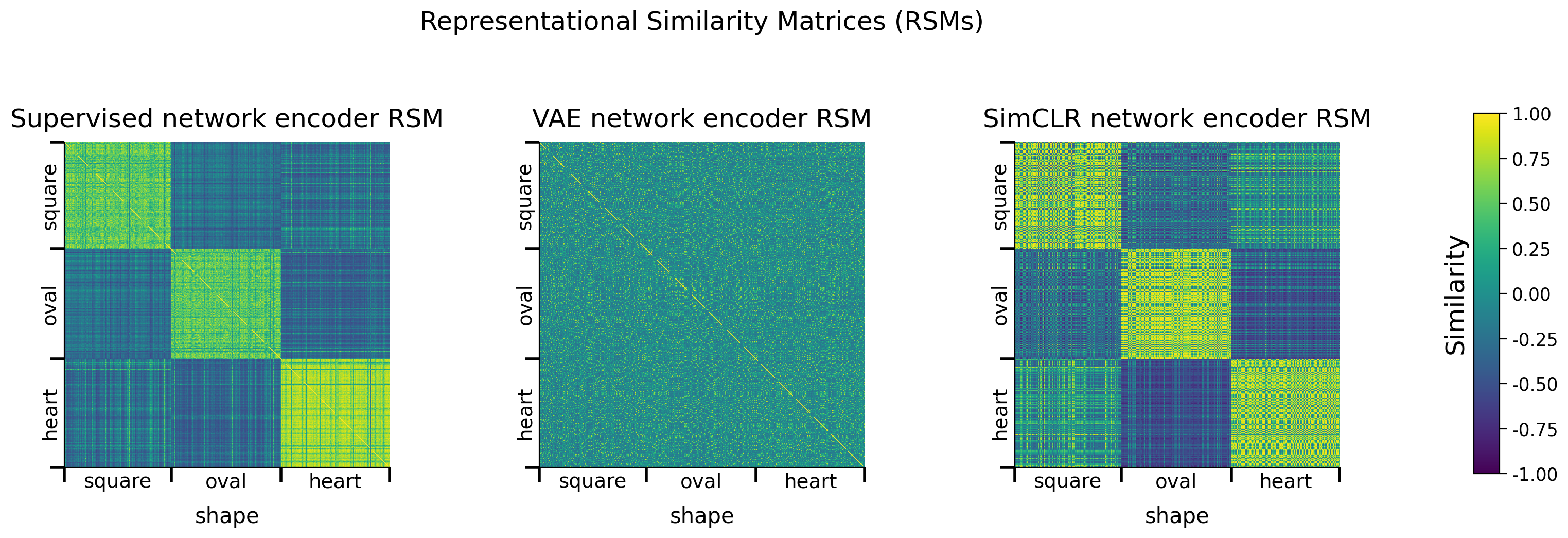
Submit your feedback#
Show code cell source
# @title Submit your feedback
content_review(f"{feedback_prefix}_SimCLR_network_encoder_RSMs_Bonus_Interactive_Demo")
Bonus Discussion 1.1.1: What can we conclude about the ability of contrastive models like SimCLR to construct a meaningful representation space?#
A. How do the pre-trained SimCLR encoder RSMs (sorted along different latent dimensions) compare to the supervised and pre-trained VAE encoder network RSMs?
B. What explains these different RSMs?
C. What advantages might some encoders have over others?
D. Does a good performance by the SimCLR encoder on a contrastive task guarantee good performance on a downstream classification task?
E. How might one modify the SimCLR encoder pre-training, for example, if the downstream task were to predict orientation instead of shape?
Supporting images for Discussion response examples for Bonus 1.1.1: All SimCLR encoder RSMs#
Show code cell source
# @markdown #### Supporting images for Discussion response examples for Bonus 1.1.1: All SimCLR encoder RSMs
Image(filename=os.path.join(REPO_PATH, "images", "rsms_simclr_encoder_60ep_bs1000_deg90_trans0-2_scale0-8to1-2_seed2021.png"), width=1000)
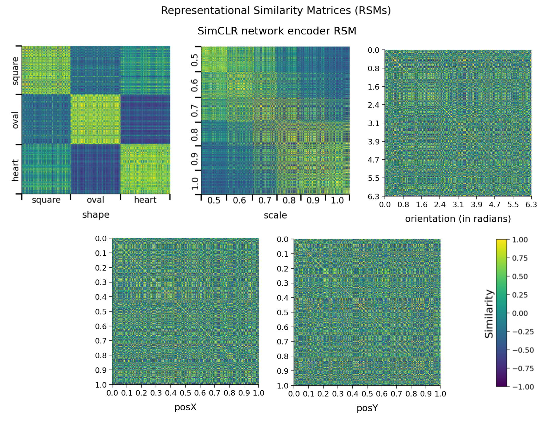
Submit your feedback#
Show code cell source
# @title Submit your feedback
content_review(f"{feedback_prefix}_Contrastive_models_Bonus_Discussion")
Bonus 2: Avoiding representational collapse#
Video 10: Avoiding Representational Collapse#
Submit your feedback#
Show code cell source
# @title Submit your feedback
content_review(f"{feedback_prefix}_Avoiding_Representational_Collapse_Bonus_Video")
Bonus 2.1: The effects of reducing the number of negative examples used in the SimCLR contrastive loss#
As seen above in the contrastive loss implementation, a strategy used to train neural networks with contrastive losses is to use large batch sizes (here, we used 1,000 examples per batch), and to use the representations of different images in a batch as each other’s negative examples. So with a batch size of 1,000, each image has one positive paired image (its paired augmentation), and 999 negative paired images (every image but itself, including its own paired augmentation, again). This enables the contrastive loss to obtain a good estimate of the full representational similarity distribution.
To observe the consequences of sampling using fewer negative examples in the contrastive loss, we use a pre-trained SimCLR network again. However, this one was pre-trained with a parameter called neg_pairs set to 2. Under the hood, this parameter affects only the contrastive loss calculation, allowing it to use only 2 of the total available negative pairs in a batch, for each image.
The following code:
Loads the parameters of a SimCLR network pre-trained on the SimCLR contrastive task, but with only 2 negative pairs used per image in the loss calculation, using
load.load_encoder(),Plots the RSMs of a few network encoders for comparison.
# Call this before any dataset/network initializing or training,
# to ensure reproducibility
set_seed(SEED)

# Load SimCLR encoder pre-trained on the contrastive loss
simclr_encoder_neg_pairs = load.load_encoder(
    REPO_PATH, model_type="simclr", neg_pairs=2
    )
Random seed 2021 has been set.
Loading SimCLR encoder from 'neuromatch_ssl_tutorial/checkpoints/simclr_encoder_2neg_60ep_bs1000_deg90_trans0-2_scale0-8to1-2_seed2021.pth'.
    => trained for 60 epochs (batch_size of 1000) on the full dSprites subset dataset
with 2 negative pairs per image used in the contrastive loss, and
with the following random affine transforms:
	degrees=90
	translation=(0.2, 0.2)
	scale=(0.8, 1.2).
Bonus Coding Exercise 2.1.1: Visualizing the network encoder RSMs, organized along different latent dimensions, and plotting similarity histograms#
We will now compare the RSM for the pre-trained SimCLR encoder trained with only 2 negative pairs to the normal pre-trained SimCLR network encoder and the random network encoder. To help us compare the representations learned by the normal and modified SimCLR encoders, we will plot a histogram of the values that make up both RSMs.
Exercise:
Visualize the RSMs, organized along the
shapelatent dimension, and compare the patterns observed for the different encoder networks.Plot a histogram of RSM values for the normal and 2-neg-pair SimCLR network encoders.
Hint:
models.plot_model_RSMs()returns the data matrices calculated for each encoder’s RSM, in order.
def rsms_and_histogram_plot():
  """
  Function to plot Representational Similarity Matrices (RSMs) and Histograms

  Args:
    None

  Returns:
    Nothing
  """
  sorting_latent = "shape" # Exercise: Try sorting by different latent dimensions
  # EXERCISE: Visualize RSMs for the normal SimCLR, 2-neg-pair SimCLR and random network encoders.
  print("Plotting RSMs...")
  simclr_rsm, simclr_neg_pairs_rsm, random_rsm = models.plot_model_RSMs(
      encoders=[simclr_encoder, simclr_encoder_neg_pairs, random_encoder],
      dataset=dSprites_torchdataset,
      sampler=test_sampler, # To see the representations on the held out test set
      titles=["SimCLR network encoder RSM",
              f"SimCLR network encoder RSM\n(2 negative pairs per image used in loss calc.)",
              "Random network encoder RSM"], # Plot titles
      sorting_latent=sorting_latent
      )
  #################################################
  # Fill in missing code below (...),
  # then remove or comment the line below to test your implementation
  raise NotImplementedError("Exercise: Plot histogram.")
  #################################################
  # Plot a histogram of RSM values for both SimCLR encoders.
  plot_rsm_histogram(
      [..., ...],
      colors=[...],
      labels=[..., ...],
      nbins=100
      )


## Uncomment below to test your code
# rsms_and_histogram_plot()
Example output:
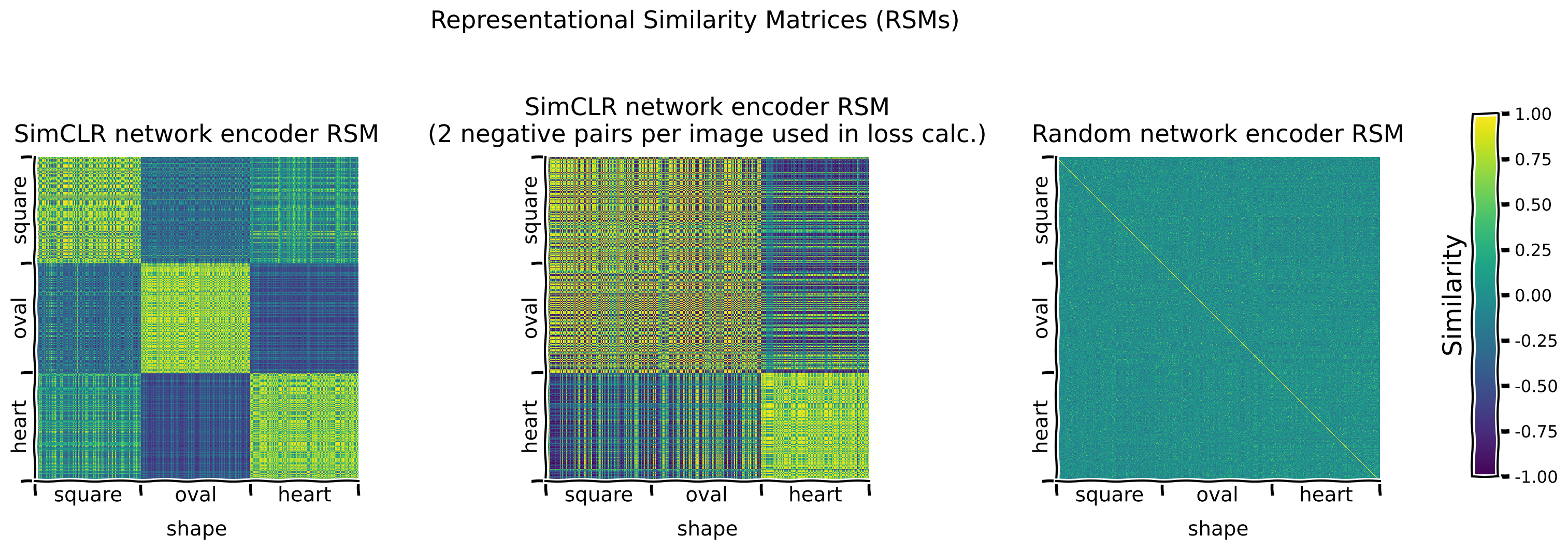
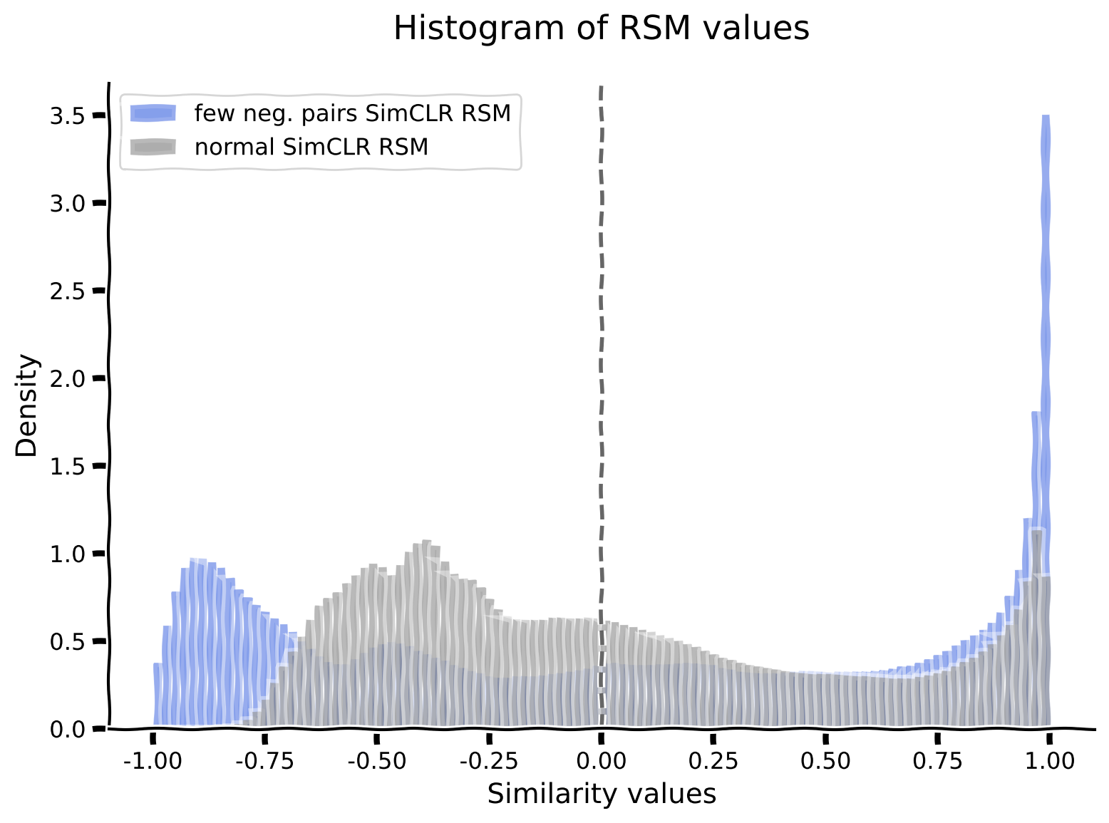
Submit your feedback#
Show code cell source
# @title Submit your feedback
content_review(f"{feedback_prefix}_Visualizing_the_network_encoder_RSMs_Bonus_Exercise")
Bonus Interactive Demo 2.1.1: Evaluating the classification performance of a logistic regression trained on the representations produced by a SimCLR network encoder pre-trained with only a few negative pairs#
For the 2-neg-pair SimCLR encoder, as the encoder parameters have already been trained, they should again be kept frozen while the classifier is trained by setting freeze_features=True.
Interactive Demo: Try different numbers of epochs for which to train the classifier. (The original setting is num_epochs=25.)
# Call this before any dataset/network initializing or training,
# to ensure reproducibility
set_seed(SEED)
print("Training a classifier on the representations learned by the SimCLR "
      "network encoder pre-trained\nusing only 2 negative pairs per image "
      "for the loss calculation...")
_, simclr_neg_pairs_loss_array, _, _ = models.train_classifier(
    encoder=simclr_encoder_neg_pairs,
    dataset=dSprites_torchdataset,
    train_sampler=train_sampler,
    test_sampler=test_sampler,
    freeze_features=True,  # Keep the encoder frozen while training the classifier
    num_epochs=50,  # DEMO: Try different numbers of epochs
    verbose=True
    )

# Plot the loss array
fig, ax = plt.subplots()
ax.plot(simclr_neg_pairs_loss_array)
ax.set_title(("Loss of classifier trained on a SimCLR encoder\n"
"trained with 2 negative pairs only."))
ax.set_xlabel("Epoch number")
_ = ax.set_ylabel("Training loss")
Random seed 2021 has been set.
Training a classifier on the representations learned by the SimCLR network encoder pre-trained
using only 2 negative pairs per image for the loss calculation...
Network performance after 50 classifier training epochs (chance: 33.33%):
    Training accuracy: 68.16%
    Testing accuracy: 66.75%
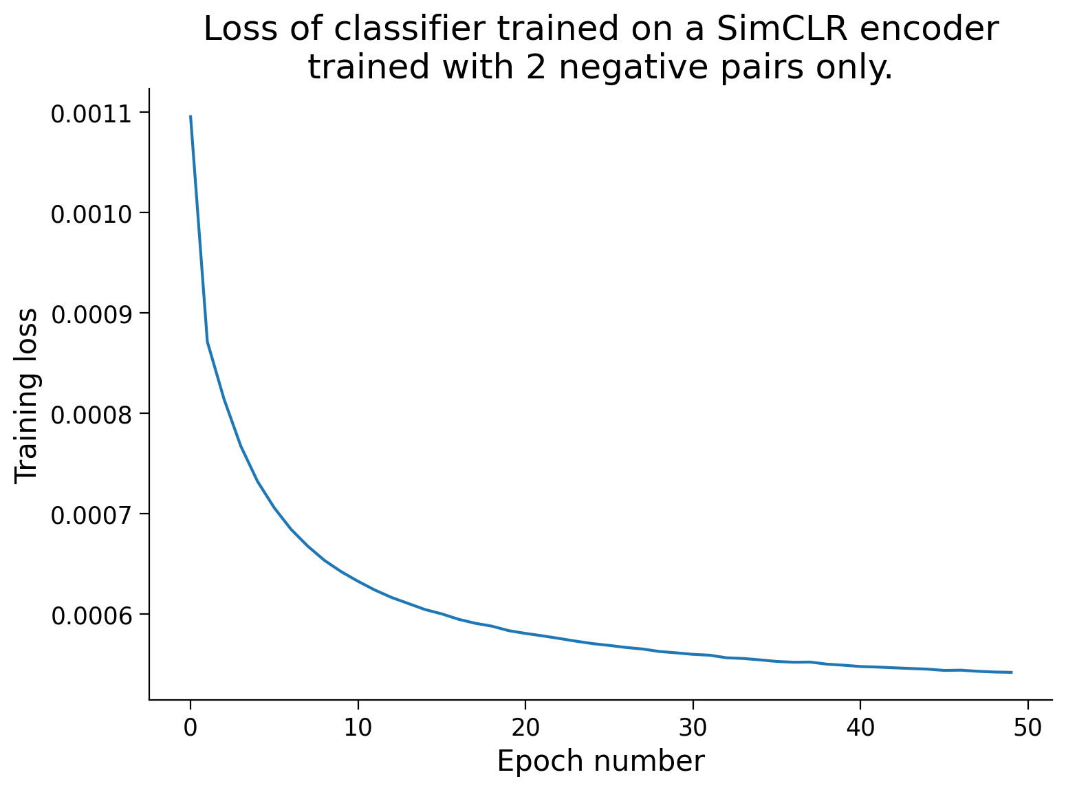
Bonus Discussion 2.1.1: What can we conclude about the importance of negative pairs in computing the contrastive loss for models like SimCLR?#
A. How does changing the number of negative pairs affect the networks’ RSMs? B. How is the shape classifier likely to perform when the encoder is pre-trained with very few negative pairs? C. What, intuitively, is the role of negative pairs in shaping the feature space that a contrastive model learns, and how does this role relate to the role of positive pairs?
Supporting images for Discussion response examples for Bonus 2.1.1: All SimCLR encoder (2 neg. pairs) RSMs#
Show code cell source
# @markdown #### Supporting images for Discussion response examples for Bonus 2.1.1: All SimCLR encoder (2 neg. pairs) RSMs
Image(filename=os.path.join(REPO_PATH, "images", "rsms_simclr_encoder_2neg_60ep_bs1000_deg90_trans0-2_scale0-8to1-2_seed2021.png"), width=1000)
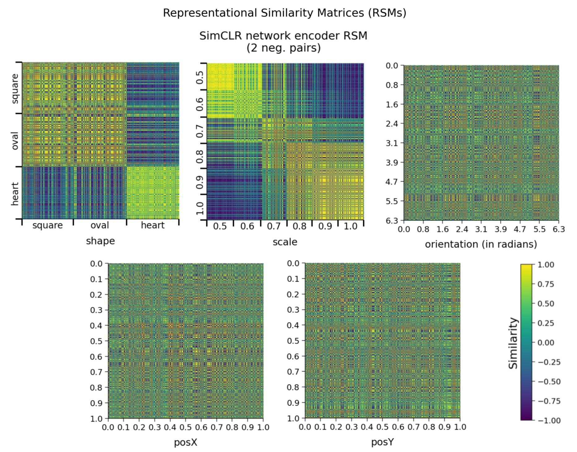
Submit your feedback#
Show code cell source
# @title Submit your feedback
content_review(f"{feedback_prefix}_Negative_pairs_in_computing_the_contrastive_loss_Bonus_Discussion")
Submit your feedback#
Show code cell source
# @title Submit your feedback
content_review(f"{feedback_prefix}_SimCLR_network_encoder_pretrained_with_only_a_few_negative_pairs_Bonus_Interactive_Demo")
After dropping the number of negative pairs used per image in pre-training a SimCLR encoder, classification accuracy drops to 66.75% on the test dataset, even after 50 classifier training epochs.
Shape classification results using different feature encoders:
Chance |
None (raw data) |
Supervised |
Random |
VAE |
SimCLR |
SimCLR (few neg.pairs) |
|
|---|---|---|---|---|---|---|---|
33.33% |
39.55% |
98.70% |
44.67% |
45.75% |
97.53% |
66.75% |
Bonus 3: Good representations enable few-shot learning#
Video 11: Few-shot Supervised Learning#
Submit your feedback#
Show code cell source
# @title Submit your feedback
content_review(f"{feedback_prefix}_FewShot_Supervised_learning_Bonus_Video")
Bonus 3.1: The benefits of pre-training an encoder network in a few-short learning scenario, i.e., when only few labelled examples are available#
The toy dataset we have been using, dSprites, is thoroughly labelled along 5 different dimensions. However, this is not the case for many datasets. Some very large datasets may have few if any labels.
One of our last steps is to examine how each of our models perform in such a case when only few labelled images are available for training. In this scenario, we will train classifiers on different fractions of the training data (between 0.01 and 1.0), and see how they perform on the test set.
For the different types of encoder, this means:
Supervised encoder: As the supervised encoder can only be trained with labels, we will start from random encoders and train them end-to-end on the classification task with the fraction of labelled images allowed. Note on * symbol: Given that that network is trained end-to-end, we will train it for more epochs, and mark it with “*” in the graphs.
Random encoder: By definition, the random encoder is untrained.
VAE encoder: As a generative model can be pre-trained on unlabelled data, we will use the VAE encoder pre-trained on the reconstruction task using the full dataset, before training the classifier layer with the fraction of labelled images allowed.
SimCLR encoder: As an SSL model can be pre-trained on unlabelled data, we will use the SimCLR encoder pre-trained on the contrastive task using the full dataset, before training the classifier layer with the fraction of labelled images allowed.
Note on number of training epochs: The numbers of epochs are specified below for when the full training dataset is used. For each fraction of the dataset a classifier is trained on, the number of training epochs is scaled up to compensate for the drop in number of training examples. For example, if we specify 10 epochs for a model, the 0.1 fraction labelled classifier will be trained over ~30 epochs. Also, we use slightly fewer epochs than above, here, in the interest of time.
Bonus Interactive Demo 3.1.1: Training classifiers on different encoders, using only a fraction of the full labelled dataset#
In this demo, we select a few fractions (4 to 6) of the full labelled dataset with which to train the classifiers.
Interactive Demo: Set labelled_fractions argument to a list of fractions (4 to 6 values between 0.01 and 1.0) with which to train classifiers for each encoder.
# Call this before any dataset/network initializing or training,
# to ensure reproducibility
set_seed(SEED)

new_supervised_encoder = models.EncoderCore()  # New, random supervised encoder

_ = models.train_encoder_clfs_by_fraction_labelled(
    encoders=[new_supervised_encoder, random_encoder, vae_encoder, simclr_encoder],
    dataset=dSprites_torchdataset,
    train_sampler=train_sampler,
    test_sampler=test_sampler,
    labelled_fractions=[0.01],  # DEMO: select 4-6 fractions to run
    num_epochs=[20, 8, 8, 8],  # Train the supervised network (end-to-end) for more epochs
    freeze_features=[False, True, True, True],  # Only train new supervised network end-to-end
    subset_seed=SEED,
    encoder_labels=["supervised", "random", "VAE", "SimCLR"],
    title="Performance of classifiers trained\nwith different network encoders",
    verbose=True
    )
Random seed 2021 has been set.
Supervised encoder: training classifiers and encoders*...
Random encoder: training classifiers...
VAE encoder: training classifiers...
SimCLR encoder: training classifiers...
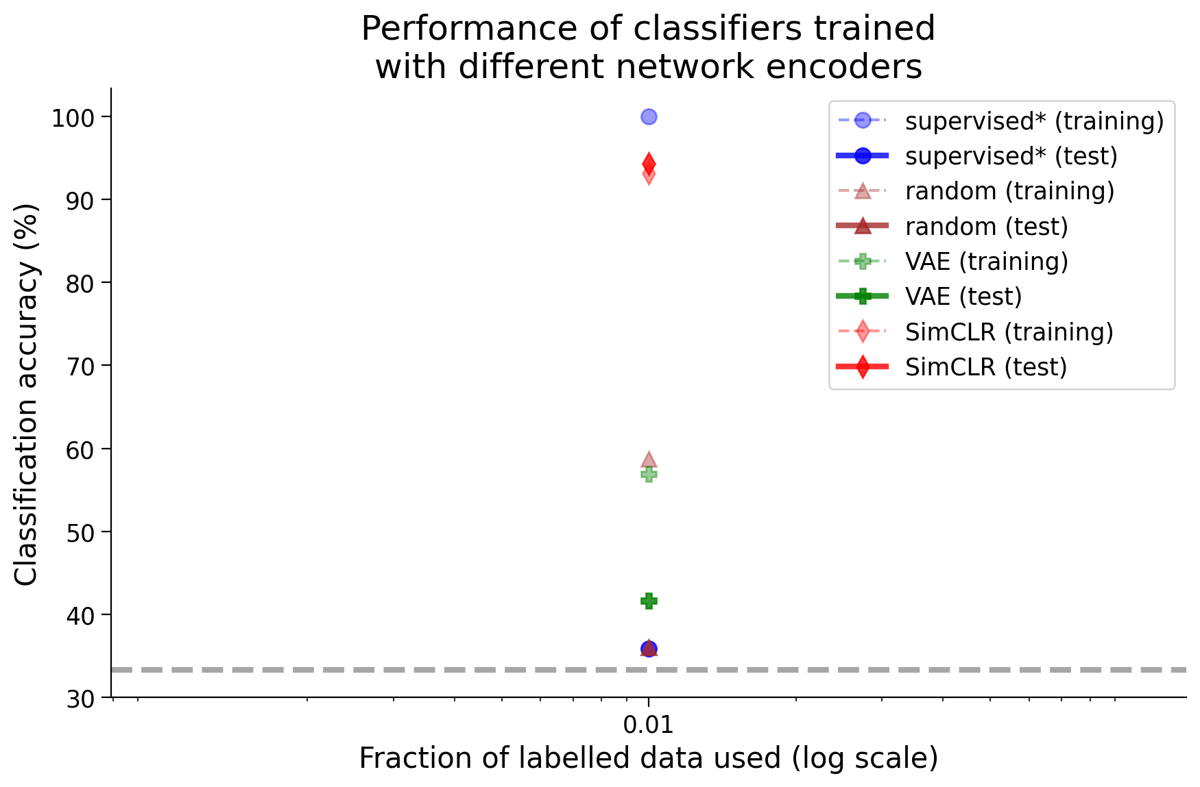
Submit your feedback#
Show code cell source
# @title Submit your feedback
content_review(f"{feedback_prefix}_Use_a_fraction_of_the_labelled_dataset_Bonus_Interactive_Demo")
Bonus Discussion 3.1.1: What can we conclude the advantages and disadvantages of the different encoder network types under different conditions?#
A. Which models are most and least affected by how much labelled data is available? B. What might explain why different models are affected differently?
Supporting images for Discussion response examples for Bonus 3.1.1: Classifier performances for various fractions of labelled data#
Show code cell source
# @markdown #### Supporting images for Discussion response examples for Bonus 3.1.1: Classifier performances for various fractions of labelled data
Image(filename=os.path.join(REPO_PATH, "images", "labelled_fractions.png"), width=600)
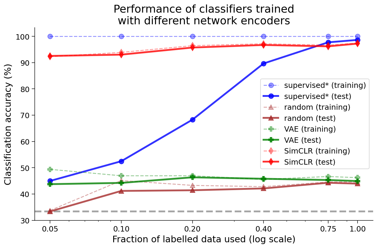
Submit your feedback#
Show code cell source
# @title Submit your feedback
content_review(f"{feedback_prefix}_Advantages_and_disadvantages_of_encoders_Bonus_Discussion")