Something Screwy - image recognition, detection, and classification of screws

Something Screwy - image recognition, detection, and classification of screws#

By Neuromatch Academy

Content creators: Joe Donovan

Production editor: Spiros Chavlis

Objective#

Useful link: NMA daily guide to projects - https://deeplearning.neuromatch.io/projects/docs/project_guidance.html

The overall goal of the project is to learn about object recognition, classification, and detection. You’ll start with simple networks, and potentially work up to larger pretained models. Your loss function is to optimize learning, not model performance.

Setup#

Install dependencies#

import os
import requests
import random
import json
import numpy as np
from skimage import io
from scipy import ndimage
from shapely.geometry import Point
from shapely.geometry.polygon import Polygon

import torch
from torch import nn
import torch.optim as optim
from torchsummary import summary
import torchvision
import torchvision.transforms as transforms

Helper functions#

Choose device#

Figure settings#

device = set_device()

GPU is enabled in this notebook. 
If you want to disable it, in the menu under `Runtime` -> 
`Hardware accelerator.` and select `None` from the dropdown menu

Data loading#

Let’s start by downloading the data and taking a look at it

Properly understanding and exploring the structure of your data is a crucial step to any project

# Download dataset, took around 4 minutes for me
# 'https://www.mvtec.com/company/research/datasets/mvtec-screws'
import requests, tarfile

url = 'https://osf.io/ruca6/download'
tarname = 'mvtec_screws_v1.0.tar.gz'
if not os.path.isfile(tarname):
  print('Data archive downloading...')
  r = requests.get(url, stream=True)
  with open(tarname, 'wb') as fd:
    fd.write(r.content)
  print('Download completed.')

# unpack tar datafile
datapath = 'screwdata'
if not os.path.exists(datapath):
  with tarfile.open(tarname) as tar:
    tar.extractall(datapath)
  os.remove(tarname)

Data archive downloading...
Download completed.

# Some json files and a folder full of images
os.listdir(datapath)

['images',
 'mvtec_screws_train.json',
 'mvtec_screws.hdict',
 'mvtec_screws_train.hdict',
 'mvtec_screws.json',
 'mvtec_screws_splitted.hdict',
 'mvtec_screws_val.json',
 'mvtec_screws_val.hdict',
 'README_v1.0.txt',
 'mvtec_screws_test.hdict',
 'mvtec_screws_test.json']

# There's some details in the readme
with open('screwdata/README_v1.0.txt') as f:
  file_contents = f.read()
  print(file_contents)

*******************************************
* MVTec Screws V1.0                       *
*                                         *
* Author: MVTec Software GmbH, July 2020. *
*         https://www.mvtec.com           *
*******************************************

All files are as in the MVTec Screws example dataset for oriented object detection, released with
HALCON version 19.05. The state of the dataset and images is as of release version 20.05.

***********
* License *
***********

The dataset, i.e. the images and the annotations, are licensed under the creative commons
Attribution-NonCommercial-ShareAlike 4.0 International (CC BY-NC-SA 4.0) license. See
https://creativecommons.org/licenses/by-nc-sa/4.0/ for more information.
For using the data in a way that falls under the commercial use clause of the license,
please contact us.

***************
* Attribution *
***************

If you use this dataset in scientific work, please cite our paper:

Markus Ulrich, Patrick Follmann, Jan-Hendrik Neudeck: 
A comparison of shape-based matching with deep-learning-based object detection;
in: Technisches Messen, 2019, DOI 10.1515/teme-2019-0076.

************
* Content: *
************

MVTec Screws contains 384 images of 13 different types of screws and nuts on a wooden background.
The objects are labeled by oriented bounding boxes and their respective category. Overall, there
are 4426 of such annotations.
The exemplary splits are those that have been used in the above mentioned publication. Initially,
they have been selected randomly, such that approximately 70% of the instances of each category are
within the training split, and 15% each in the validation and test splits.

* folder images contains the screw images.
* mvtec_screws.json contains the annotations for all images in COCO format.
* mvtec_screws_train/val/test.json contain examplary splits as mentioned above, in COCO format.
* mvtec_screws.hdict contains the DLDataset unsplitted.
* mvtec_screws_split.hdict contains the DLDataset with splits.

******************************
* Usage of DLDataset-format: *
******************************

The .hdict files can be used within HALCON by reading them, e.g. via

read_dict (<path_to_mvtec_screws.hdict>, [], [], DLDataset)

The image path has to be set to the location of the images folder <path_to_images_folder> by

set_dict_tuple(DLDataset, 'image_dir', <path_to_images_folder>)

To store this information within the dataset, the dataset should be written by
write_dict (DLDataset, <path_to_mvtec_screws.hdict>, [], [])

In HALCON object detection we use subpixel-precise annotations with a pixel-centered coordinate-system, i.e.
the center of the top-left corner of the image is at (0.0, 0.0), while the top-left corner of the image is
located at (-.5, -.5). Note that when used within HALCON the dataset does not need to be converted, as this
format is also used within the deep learning based object detection of HALCON.

***************
* COCO Format *
***************

MVTec screws is a dataset for oriented box detection. We use a format that is very similar to that of the
COCO dataset (cocodataset.org). However, we need 5 parameters per box annotation to store the orientation.
We use the following labels.

Each box contains 5 parameters (row, col, width, height, phi), where

* 'row' is the subpixel-precise center row (vertical axis of the coordinate system) of the box.
* 'col' is the subpixel-precise center column (horizontal axis of the coordinate system) of the box.
* 'width' is the subpixel-precise width of the box. I.e. the length of the box parallel to the orientation 
  of the box.
* 'height' is the subpixel-precise width of the box. I.e. the length of the box perpendicular to the
  orientation of the box.
* 'phi' is the orientation of the box in radian, given in a mathematically positive sense and with respect
  to the horizontal (column) image axis. E.g. for phi = 0.0 the box is oriented towards the right side of 
  the image, for phi = pi/2 towards the top, for phi = pi towards the left, and for phi=-pi/2 towards the 
  bottom. Phi is always in the range (-pi, pi].

Note that width and height are defined in contrast to the DLDataset format in HALCON, where we use 
semi-axis lengths.

Coordinate system: In comparison to the pixel-centered coordinate-system of HALCON mentioned above,
                   for COCO it is common to set the origin to the top-left-corner of the top-left
				   pixel, hence in comparison to the DLDataset-format, (row,col) are shifted by (.5, .5).

#Load the json file with the annotation metadata
with open(os.path.join(datapath, 'mvtec_screws.json')) as f:
  data = json.load(f)

print(data.keys())
print(data['images'][0])
print(data['annotations'][0])

dict_keys(['categories', 'images', 'annotations', 'licenses', 'info'])
{'file_name': 'screws_001.png', 'height': 1440, 'width': 1920, 'id': 1, 'license': 1}
{'area': 3440.97, 'bbox': [184.5, 876.313, 55, 62.5631, 0], 'category_id': 7, 'id': 1001, 'image_id': 1, 'is_crowd': 0}

#Load the images, and make some helpful dict to map the data
imgdir = os.path.join(datapath, 'images')

#remap images to dict by id
imgdict = {l['id']:l for l in data['images']}
#read in all images, can take some time
for i in imgdict.values():
  i['image'] = io.imread(os.path.join(imgdir, i['file_name']))[:, :,: 3]  # drop alpha channel, if it's there

# remap annotations to dict by image_id
from collections import defaultdict
annodict = defaultdict(list)
for annotation in data['annotations']:
  annodict[annotation['image_id']].append(annotation)

# setup list of categories
categories = data['categories']
ncategories = len(categories)
cat_ids = [i['id'] for i in categories]
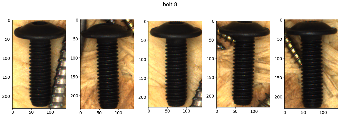
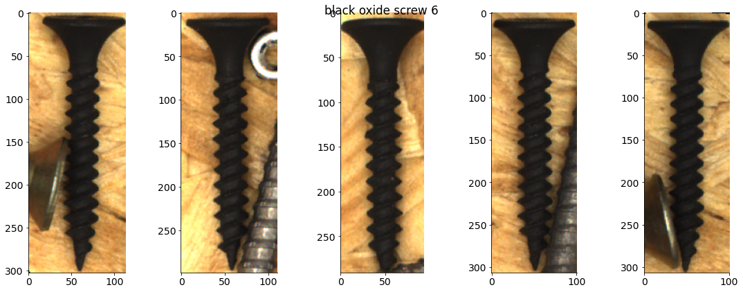
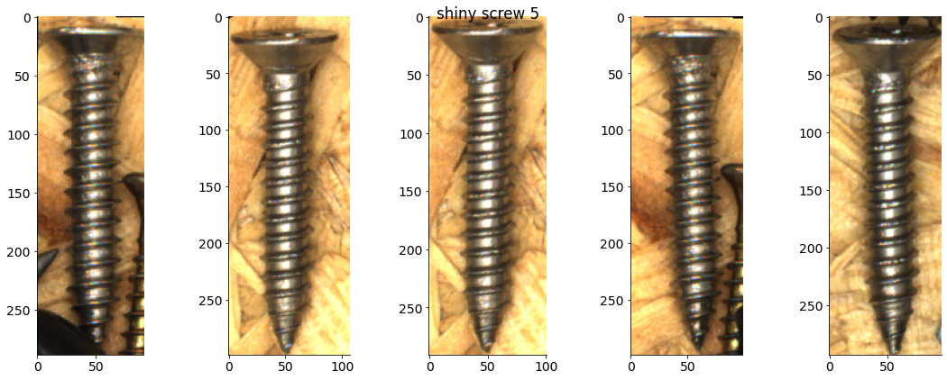
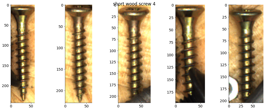
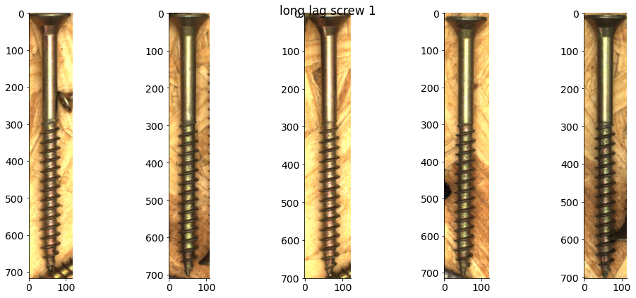
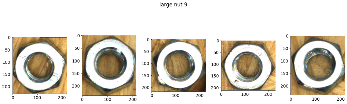
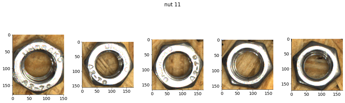
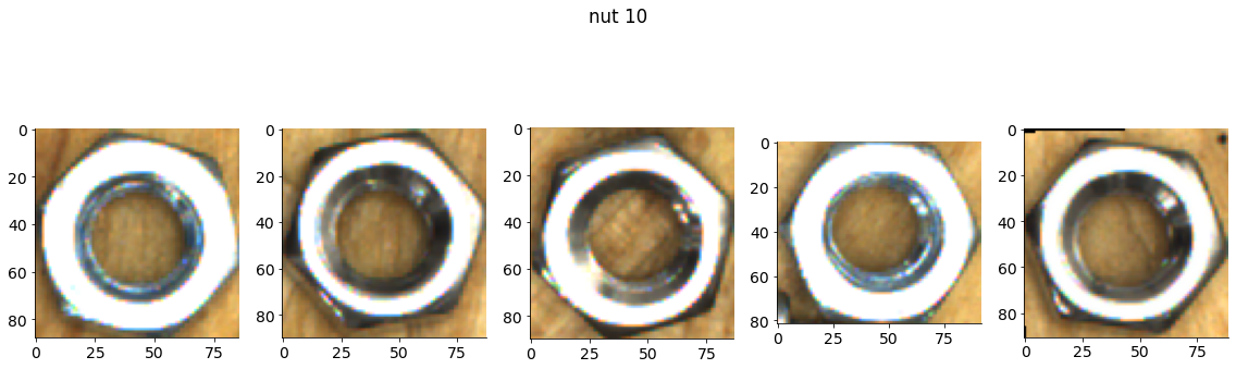
category_names = {7:'nut', 3:'wood screw', 2:'lag wood screw', 8:'bolt',
                  6:'black oxide screw', 5:'shiny screw', 4:'short wood screw',
                  1:'long lag screw', 9:'large nut', 11:'nut', 10:'nut',
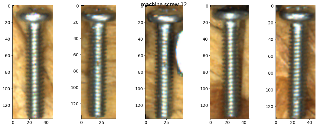
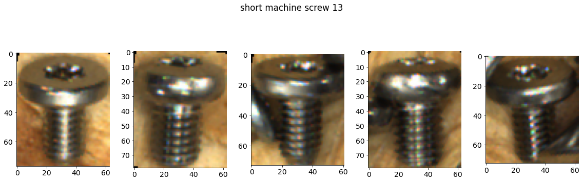
                  12:'machine screw', 13:'short machine screw' }

Let’s check out some data#

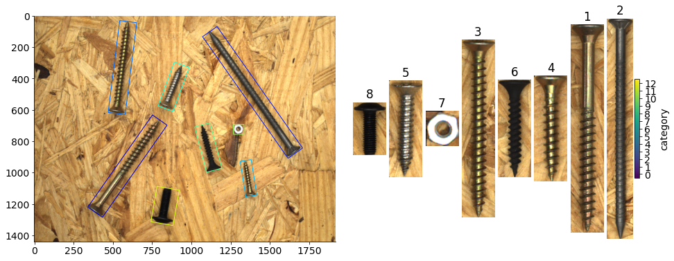
# Let's look at one image and it's associated annotations
imageid = 100
im = imgdict[imageid]['image']
gs = gridspec.GridSpec(1, 1 + len(annodict[imageid]),
                       width_ratios=[1,]+[.1]*len(annodict[imageid]),
                       wspace=.05)
plt.figure()
ax = plt.subplot(gs[0])
plt.imshow(im)
cmap_normal = plt.Normalize(0, ncategories)

for i, annotation in enumerate(annodict[imageid]):
  bbox = annotation['bbox']

  # plt.scatter(*rot_center)
  # plt.scatter(*corner_points.T, c='r')

  ax = plt.subplot(gs[0])
  color = plt.cm.jet(cmap_normal(annotation['category_id']))
  rect = patches.Rectangle((bbox[1] - bbox[3]/2 ,
                            bbox[0] - bbox[2]/2), bbox[3], bbox[2],
                           linewidth=1, edgecolor=color, facecolor='none')
  t = plt_transforms.Affine2D().rotate_around(bbox[1], bbox[0], -bbox[4]+np.pi/2)
  rect.set_transform(t + plt.gca().transData)
  ax.add_patch(rect)

  plt.subplot(gs[i + 1])
  rotated_im = extract_subimg_bbox(im, bbox)
  plt.imshow(rotated_im)
  plt.axis('off')
  plt.title(annotation['category_id'])

plt.colorbar(ticks=range(ncategories), label='category')
plt.clim(-0.5, ncategories - .5)
plt.show()

../../_images/6ef02116a1f3a28434dcdd908b81f4b7da7b64fc9d02ebd5853ed3a7f31f446f.png

# create a dict mapping category id to all subimages, can take some time to run
cat_imgdict = defaultdict(list)
for img_id, image in imgdict.items():
  for annotation in annodict[img_id]:
    bbox = annotation['bbox']
    subimg = extract_subimg_bbox(image['image'], bbox)
    cat_imgdict[annotation['category_id']].append(subimg.copy())

# How many images are in each category?
for k, v  in cat_imgdict.items():
  print(f"Category ID {k} has {len(v)} items")  #f-strings are neat - see https://realpython.com/python-f-strings/

Category ID 7 has 365 items
Category ID 3 has 317 items
Category ID 2 has 314 items
Category ID 8 has 367 items
Category ID 6 has 393 items
Category ID 5 has 387 items
Category ID 4 has 315 items
Category ID 1 has 313 items
Category ID 9 has 320 items
Category ID 11 has 346 items
Category ID 10 has 347 items
Category ID 12 has 322 items
Category ID 13 has 321 items

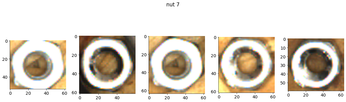
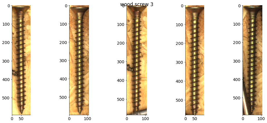
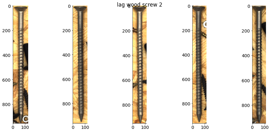
# Plot some examples from each category
for catid, examples in cat_imgdict.items():
  num_examples = 5
  gs = gridspec.GridSpec(1, num_examples)
  plt.figure()
  for i, example in enumerate(examples[:num_examples]):
    plt.subplot(gs[i])
    plt.imshow(example)
    plt.suptitle(f"{category_names[catid]} {catid}")

../../_images/ee38563ef324078b0a7d902e7585017f4a41ec14f160755a29d3448cc927d384.png

../../_images/ae60e03cf2acacc9e00d10054062c3f57200bbe4dc0b81b7de206357bfd8e629.png

../../_images/5c1f331cc1d0600bcf146aaeea41d862bb34e6723c10b6645db334271d69ad45.png

../../_images/87485d8e06f7becc5d027d7eec1975501471b83ac2041904d030a78e4c5c3572.png

../../_images/7ec1d55bc5b20f2068133c7271bce7d99df3cf9fb078fce17963e2f3f2750289.png

../../_images/a2b1d7e86e0625302a9b179271a3c9e72b7ecafa13698bdd21a8436e1e07a077.png

../../_images/6b55f88cda350ff13ee85192504d28621f1e772f33153915902b1755ad121e57.png

../../_images/6fcdfac6a357d2fd4b006b5db300756719c947266a8f9eb197084f17152c9497.png

../../_images/22f0e326bf5a645d0e22ba8966216f58a0840b08bc55ade9f3aaf0d1afa0ef8f.png

../../_images/2d4e3721f83bb276defffec22919b4e8b9c93b5ae59b3ffdd19c40769aca690a.png

../../_images/1253a1dee2d1e954060cf3e6f331895354de3e24a157ea497dfcc7c62848948e.png

../../_images/9f77e1243b7f8cde053dd17a4db9010b2fe18e3a6bf82e313b0bb84359a3cbf0.png

../../_images/d8e3c4036f5c8edc291723b041fb121eccf5afa88592949e5c202f9f8b7099ba.png

Object classification#

Setting up for our first challenge#

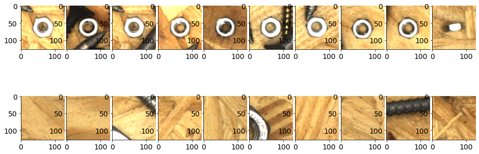
The challenge of detecting hetergogenously sized objects scattered throughout an image can be challenging, so let’s start with something simpler - detecting whether a fixed sized image contains a nut or is blank.

# Start with fixed sized patches that either have a screw or not
use_categories = [7, 10]
# for screw patches use categories that have smaller bounding boxes
patch_size = np.array((128, 128))
num_patches_per_category = 500

nut_patches = []
for img_id, image in imgdict.items():
  for annotation in annodict[img_id]:
    if annotation['category_id'] in use_categories:
      bbox = annotation['bbox']
      rot_center, width, height, theta = unpack_bbox(bbox)
      subimg = extract_subimg(image['image'], rot_center, patch_size[0], patch_size[1], 0)
      if all(subimg.shape[:2] == patch_size):
        nut_patches.append(subimg)
      # plt.figure()
      # plt.imshow(subimg)

  if len(nut_patches) >= num_patches_per_category:
    break

#Select random blank patches
blank_patches = []
for i in range(len(nut_patches)):
  while True: #until a suitable random patch is found
    #choose random image
    imgid, imgobj = random.choice(list(imgdict.items()))
    im = imgobj['image']
    #choose random place at least half a patch size from edges
    rand_center = np.random.randint((patch_size//2), np.array(im.shape)[:2] - patch_size//2)
    corners = rotcorners_from_coords(rand_center, patch_size[0], patch_size[1], 0)
    #check if the random patch intersects with any labeled objects
    if not any([Polygon(corners).intersects(Polygon(rotcorners_from_coords(*unpack_bbox(annotation['bbox'])))) for annotation in annodict[imgid]]):
      rand_patch = im[rand_center[0]-patch_size[0]//2:rand_center[0]+patch_size[0]//2, rand_center[1]-patch_size[1]//2:rand_center[1]+patch_size[1]//2]
      blank_patches.append(rand_patch)
      break

# TODO seems like rarely the patches aren't fully blank - are some labels missing??

# could also use some images from cifar etc.
num_examples = 10
plt.figure()
gs = gridspec.GridSpec(2, num_examples, wspace=.05)
for i in range(num_examples):
  plt.subplot(gs[0, i])
  plt.imshow(nut_patches[i])
  plt.subplot(gs[1, i])
  plt.imshow(blank_patches[i])

patch_labels = [1,]*len(nut_patches) + [0,]*len(blank_patches)  #1 if nut
all_patches = nut_patches + blank_patches #list concat

# randomly shuffle
shuffle_idx = np.random.choice(len(patch_labels), len(patch_labels), replace=False)
patch_labels = [patch_labels[i] for i in shuffle_idx]
all_patches = [all_patches[i] for i in shuffle_idx]

../../_images/826940452b6381b306ffcaa8ec89d5b2bf6c88d7f99c296f1d88f438146db0f1.png

# Check shapes are correct
# assert all([p.shape == (128,128,3) for p in all_patches])
[i for i,p in enumerate(all_patches) if p.shape != (128, 128, 3)]

[]

Preparing our first network#

Before immediately jumping into coding a network, first think about what the structure of the network should look like. Hint - it’s often helpful to start thinking about the shape/dimensionality of the inputs and outputs

# Preprocess data
preprocess = transforms.Compose([
   transforms.ToTensor(),
   transforms.Normalize(mean=[0.485, 0.456, 0.406], std=[0.229, 0.224, 0.225])
])

train_frac = .2
train_number = int(len(all_patches)*train_frac)
# test_nuumber = all_patches.len()-train_number
train_patches, train_labels = all_patches[:train_number], patch_labels[:train_number]
test_patches, test_labels = all_patches[train_number:], patch_labels[train_number:]

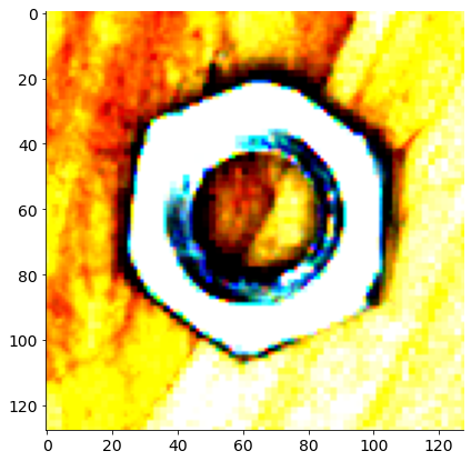
plt.figure()
plt.imshow(preprocess(all_patches[0]).permute(1, 2, 0))
plt.show()

../../_images/1cb61c31cee9b6f7052670053982f5e814325aea7bc225f1e285e14be4c72f4f.png

class SimpleScrewNet(nn.Module):
  def __init__(self):
    super().__init__()

    LeakyReLU = nn.LeakyReLU()
    MaxPool2d = nn.MaxPool2d(2, stride=2)
    self.layers = nn.Sequential(
        nn.Conv2d(3, 16, kernel_size=7, stride=2),
        LeakyReLU,
        MaxPool2d,

        nn.Conv2d(16, 32, kernel_size=5),
        # nn.Conv2d(32, 32, kernel_size=5),
        LeakyReLU,
        MaxPool2d,

        nn.Conv2d(32, 64, kernel_size=5),
        LeakyReLU,
        MaxPool2d,

        nn.Flatten(1),

        nn.Linear(1024, 64),
        # nn.Dropout(),
        nn.Linear(64, 2),

        # nn.Conv2d(3, 6, 5),
        # nn.MaxPool2d(2, 2),
        # nn.Conv2d(6, 16, 5),
        # nn.Linear(16 * 5 * 5, 120),
        # nn.Linear(120, 84),
        # nn.Linear(84, 2),

    )

  def forward(self, x):
    # Simply pass the data through the layers
    return self.layers(x)

# Inspect model structure and layer sizes
snet = SimpleScrewNet().to(device)
summary(snet, input_size=(3, 128, 128))

----------------------------------------------------------------
        Layer (type)               Output Shape         Param #
================================================================
            Conv2d-1           [-1, 16, 61, 61]           2,368
         LeakyReLU-2           [-1, 16, 61, 61]               0
         MaxPool2d-3           [-1, 16, 30, 30]               0
            Conv2d-4           [-1, 32, 26, 26]          12,832
         LeakyReLU-5           [-1, 32, 26, 26]               0
         MaxPool2d-6           [-1, 32, 13, 13]               0
            Conv2d-7             [-1, 64, 9, 9]          51,264
         LeakyReLU-8             [-1, 64, 9, 9]               0
         MaxPool2d-9             [-1, 64, 4, 4]               0
          Flatten-10                 [-1, 1024]               0
           Linear-11                   [-1, 64]          65,600
           Linear-12                    [-1, 2]             130
================================================================
Total params: 132,194
Trainable params: 132,194
Non-trainable params: 0
----------------------------------------------------------------
Input size (MB): 0.19
Forward/backward pass size (MB): 1.48
Params size (MB): 0.50
Estimated Total Size (MB): 2.18
----------------------------------------------------------------

# Loss
loss_fn=nn.CrossEntropyLoss()
optimizer=optim.SGD(snet.parameters(),lr=0.000001,momentum=0.3)

# Train
num_epoch = 5
train_losses= []  # loss per epoch
test_losses= []  # loss per epoch
test_corrects = []  # % correct per epoch

test_correct = []
with torch.no_grad():
  for img,lbl in zip(test_patches, test_labels):
    img=torch.from_numpy(img).float().permute(2,1,0).unsqueeze(0).cuda()
    lbl=torch.torch.as_tensor(lbl).unsqueeze(0).cuda()
    predict=snet(img)
    test_correct.append((predict.argmax() == lbl).item())
test_correct = np.array(test_correct)
print(f'Before starting: {test_correct.mean()*100:.2f}% of test images correct')

for epoch in range(num_epoch):
  train_loss=0.0
  test_loss=0.0
  test_correct = []

  snet.train()
  # for img,lbl in train_ds_loader:
  for img,lbl in zip(train_patches, train_labels):
    img=torch.from_numpy(img).float().permute(2,1,0).unsqueeze(0).cuda()
    lbl=torch.torch.as_tensor(lbl).unsqueeze(0).cuda()

    optimizer.zero_grad()
    # print(img.shape)
    predict=snet(img)
    loss=loss_fn(predict,lbl)
    loss.backward()
    optimizer.step()
    train_loss+=loss.item()*img.size(0)

  with torch.no_grad():
    for img,lbl in zip(test_patches, test_labels):
      img=torch.from_numpy(img).float().permute(2,1,0).unsqueeze(0).cuda()
      lbl=torch.torch.as_tensor(lbl).unsqueeze(0).cuda()
      predict=snet(img)
      loss=loss_fn(predict,lbl)
      test_loss+=loss.item()*img.size(0)
      test_correct.append((predict.argmax() == lbl).item())

  test_correct = np.array(test_correct).mean()
  train_losses.append(train_loss)
  test_losses.append(test_loss)
  test_corrects.append(test_correct)
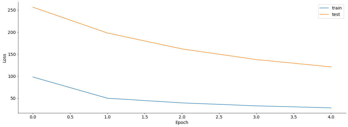
  print('Epoch:{} Train Loss:{:.3f} Test Losss:{:.3f} Percent correct: {:.2f}%'.format(epoch,train_loss,test_loss, test_correct*100))

Before starting: 50.37% of test images correct
Epoch:0 Train Loss:97.973 Test Losss:256.380 Percent correct: 93.27%
Epoch:1 Train Loss:49.839 Test Losss:197.818 Percent correct: 96.51%
Epoch:2 Train Loss:39.270 Test Losss:161.713 Percent correct: 97.26%
Epoch:3 Train Loss:32.547 Test Losss:137.508 Percent correct: 98.38%
Epoch:4 Train Loss:27.970 Test Losss:120.993 Percent correct: 98.38%

# calculate percentage correct
correct = []
with torch.no_grad():
  for img,lbl in zip(test_patches, test_labels):
    img=torch.from_numpy(img).float().permute(2,1,0).unsqueeze(0).to(device)
    lbl=torch.torch.as_tensor(lbl).unsqueeze(0).to(device)
    predict=snet(img)
    correct += [(predict.argmax() == lbl).item()]
correct = np.array(correct)
print(f'{correct.mean():.3f}% of test images correct')

0.984% of test images correct

plt.figure()
plt.plot(train_losses, label='train')
plt.plot(test_losses, label='test')
plt.legend()
plt.xlabel('Epoch')
plt.ylabel('Loss')

Text(0, 0.5, 'Loss')

../../_images/5698e67e08bd26849cfa8845648c5f4fa7da9ab168a6b4e2523d2e454ab5f3c6.png

Damaged screw detection#

There’s a dataset with anamolous screws on Kaggle - https://www.kaggle.com/ruruamour/screw-dataset

Download and inspect the dataset, then setup a network for classification of damaged or normal screw

import json, os
# Here's a code snippet for downloading from kaggle
dirname = '~/.kaggle/' 
os.mkdir(dirname)

file_path = f"{dirname}{'kaggle.json'}"
# create an empty file
with open(file_path, 'w') as fp:
  pass

# create/download api token from Kaggle -> upper right side -> account -> API -> create API token, and copy it here
api_token = {"username":"username here","key":"enter api key here"}

with open('/root/.kaggle/kaggle.json', 'w') as file:
  json.dump(api_token, file)

# chnage permissions
s = '600'
os.chmod(file_path, int(s, base=8))

# download
!kaggle datasets download -d ruruamour/screw-dataset

Multi-class classification#

So far we’ve been doing object classification on single classes from the dataset. Change your network to use the 13 classes from the original dataset to classify images of fixed sized into the 13 classes. Note that not all classes are the same sized, so you’ll have to use larger image patches and likely change the configuration of your network some.

# Reminder, you can use extract_subimg(im, rot_center, width, height, theta) to extract image patches

Object detection#

Object classification of fixed sized images with a single item is nice, but for many real world tasks detection of multiple objects throughout an image is crucial. Now we will try to create a network for object detection.

Here’s a useful intro to some of the different types of object classification tasks: https://machinelearningmastery.com/object-recognition-with-deep-learning/

First start by thinking about how the network could capture the location of multiple objects - a single classifer layer at the end of the network won’t be enough. The YOLO paper might be a helpful read as well as this algorithm comparison. Try to implement your own network (keep in mind for a practice training time you won’t be able to use as deep of a network as many of the papers).

Network performance/introspection#

An important skill for deep learning, as well as any data or programming task is to know how to inspect and debug the performance of your system. Check out what your intermediate layers are actually learning - does this give you any hints to improve your performance? The W1D2 tutorial might also be useful.

Oriented bounding boxes#

The standard yolo just draws bounding boxes, and doesn’t handle rotated objects elegantly.

There’s several works that extend yolo with oriented boxes or have other network structures that can produce oriented bounding boxes(see here).

Class clustering#

We’ve been using provided labels to define our object classes (a form of supervised learning). For many datasets you won’t labels or they will be incomplete.

Try unsupervised clustering to segment the data into groups. Either classical approaches which sklearn will be very helpful for, or using deep learning approaches (example 1, example 2).

How do the unsupervised clusters compare with the provided labels?

Perspective and scale#

Transfer Learning#

There’s many models for object detection/segmentation, for instance: yolo3 minimal, yolov5, detetectron2, Scaled-YOLOv4.

I’d recommend reading the original YOLO paper and then starting with yolo3 minimal (less performance, but more readable code than the more complicated frameworks).

Starting from one of these pretrained networks train it on your screw dataset. How does it’s performance compare to your simpler network’s performance?

Useful links#

Library of open 3D cad models of bolts etc.: https://www.bolts-library.org/en/index.html