Data Augmentation in image classification models

Data Augmentation in image classification models#

By Neuromatch Academy

Content creators: Jama Hussein Mohamud, Alex Hernandez-Garcia

Production editors: Spiros Chavlis, Saeed Salehi

Objective#

Data augmentation refers to synthetically increasing the amount of training data by transforming the existing training examples. Data augmentation has been shown to be a very useful technique, especially in computer vision applications. However, there are multiple ways of performing data augmentation and it is yet to be understood which transformations are more effective and why, and how data augmentation interacts with other techniques. In fact, it is common to see different augmentation schemes and setups in different papers. For example, there are perceptually possible image transformations (related to human visual perception), simple synthetic transformations such as cutout, more artificial transformations such as mixup that even transform the class labels, among many others.

In this notebook, we will show how to train deep neural networks for image classification with data augmentation and analyse the results.

Setup#

Install dependencies#

# imports
import os
import csv
import multiprocessing

import numpy as np
import pandas as pd
import matplotlib.pyplot as plt

import torch
import torch.nn as nn
import torch.optim as optim
import torch.nn.functional as F
import torch.backends.cudnn as cudnn
from torch.autograd import Variable

import torchvision
import torchvision.transforms as transforms

Set random seed#

Executing set_seed(seed=seed) you are setting the seed

Set device (GPU or CPU)#

set_seed(seed=2021)
set_device()

Random seed 2021 has been set.
GPU is enabled in this notebook.

'cuda'

Training hyperparameters#

Note: We have reduced the number of epochs, end_epochs. The value was set to 200. Please, change it back and run the code.

# hyper-parameters
use_cuda = torch.cuda.is_available()
alpha = 1  # alpha for mixup augmentation
best_acc = 0  # best test accuracy
start_epoch = 0  # start from epoch 0 or last checkpoint epoch
batch_size = 128
end_apochs = 15  # Please change this to 200
base_learning_rate = 0.1
cutout = True  # True/False if you want to use cutout augmentation
mixup = False  # True/False if you want to use mixup augmentation
n_holes = 1  # number of holes to cut out from image for cutout
length = 16  # length of the holes for cutout augmentation
torchvision_transforms = False  # True/False if you want use torchvision augmentations

Augmentation#

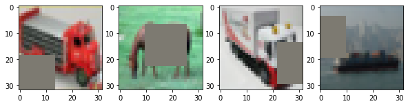
Cutout#

Randomly mask out one or more patches from an image.

Cutout Augmentation class

Mixup#

Mixup is a data augmentation technique that combines pairs of examples via a convex combination of the images and the labels. Given images \(x_i\) and \(x_j\) with labels \(y_i\) and \(y_j\), respectively, and \(\lambda \in [0, 1]\), mixup creates a new image \(\hat{x}\) with label \(\hat{y}\) the following way:

(128)#\[\begin{align} \hat{x} &= \lambda x_i + (1 - \lambda) x_j \\ \hat{y} &= \lambda y_i + (1 - \lambda) y_j \end{align}\]

You may check the original paper and code repository.

mixup_data Augmentation function

Data#

Datasets#

We will start using CIFAR-10 data set from PyTorch, but with small tweaks we can get any other data we are interested in.

Download and prepare Data

==> Preparing data...
Downloading https://www.cs.toronto.edu/~kriz/cifar-10-python.tar.gz to ./CIFAR10/cifar-10-python.tar.gz

Extracting ./CIFAR10/cifar-10-python.tar.gz to ./CIFAR10
Files already downloaded and verified

CIFAR-10#

CIFAR-10 is a data set of 50,000 colour (RGB) training images and 10,000 test images, of size 32 x 32 pixels. Each image is labelled as 1 of 10 possible classes:

'plane', 'car', 'bird', 'cat', 'deer', 'dog', 'frog', 'horse', 'ship', 'truck'

The data set is stored as a custom torchvision.datasets.cifar.CIFAR object. You can check some of its properties with the following code:

print(f"Object type: {type(trainset)}")
print(f"Training data shape: {trainset.data.shape}")
print(f"Test data shape: {testset.data.shape}")
print(f"Number of classes: {np.unique(trainset.targets).shape[0]}")

Object type: <class 'torchvision.datasets.cifar.CIFAR10'>
Training data shape: (50000, 32, 32, 3)
Test data shape: (10000, 32, 32, 3)
Number of classes: 10

# choose percentage from the trainset. set percent = 1.0 to use the whole train data
percent = 1.0
trainset = percentageSplit(trainset, percent = percent)
print(f"size of the new trainset: {len(trainset)}")

size of the new trainset: 50000

Data loaders#

A dataloader is an optimized data iterator that provides functionality for efficient shuffling, transformation and batching of the data.

# Dataloader
num_workers = multiprocessing.cpu_count()

print(f'----> number of workers: {num_workers}')

trainloader = torch.utils.data.DataLoader(
    trainset, batch_size=batch_size, shuffle=True, num_workers=num_workers)
testloader = torch.utils.data.DataLoader(
    testset, batch_size=batch_size, shuffle=False, num_workers=num_workers)

----> number of workers: 4

Visualization#

To visualize some of the augmentations, make sure you set to True their corresponding flags in the hyperparameters section

# get batch of data
batch_X, batch_Y =  next(iter(trainloader))

def plot_mixed_images(images):
  inv_normalize = transforms.Normalize(
                      mean= [-m/s for m, s in zip(mean, std)],
                      std= [1/s for s in std]
                      )
  inv_PIL = transforms.ToPILImage()
  fig = plt.figure(figsize=(10, 8))
  for i in range(1, len(images) + 1):
    image = images[i-1]
    ax = fig.add_subplot(1, 4, i)
    inv_tensor = inv_normalize(image).cpu()
    ax.imshow(inv_PIL(inv_tensor))
  plt.show()

# Mixup Visualization
if mixup:
  alpha = 0.9
  mixed_x, y_a, y_b, lam = mixup_data(batch_X, batch_Y,
                                      alpha=alpha, use_cuda=use_cuda)
  plot_mixed_images(mixed_x[:4])

# Mixup Visualization
if cutout:
  plot_mixed_images(batch_X[:4])

../../_images/38a806320f9fe59226a9a49516c7b148227c36d25e413368d6dc543a4a674593.png

# Torchvision Visualization
if torchvision_transforms:
  plot_mixed_images(batch_X[:4])

Model#

Architecture: ResNet#

ResNet is a family of network architectures whose main property is that the network is organised as a stack of residual blocks. Residual blocks consist of a stack of layers whose output is added the input, making a shortcut connection.

See the original paper for more details.

ResNet is just a popular choice out of many others, but data augmentation works well in general. We just picked ResNet for illustration purposes.

ResNet model in PyTorch

Show code cell source Hide code cell source

# @markdown ResNet model in PyTorch

class BasicBlock(nn.Module):
  """ResNet in PyTorch.
        Reference:
        [1] Kaiming He, Xiangyu Zhang, Shaoqing Ren, Jian Sun
        Deep Residual Learning for Image Recognition.
        arXiv:1512.03385
  """
  expansion = 1

  def __init__(self, in_planes, planes, stride=1):
    super(BasicBlock, self).__init__()
    self.conv1 = nn.Conv2d(in_planes, planes, kernel_size=3, stride=stride, padding=1, bias=False)
    self.bn1 = nn.BatchNorm2d(planes)
    self.conv2 = nn.Conv2d(planes, planes, kernel_size=3, stride=1, padding=1, bias=False)
    self.bn2 = nn.BatchNorm2d(planes)

    self.shortcut = nn.Sequential()
    if stride != 1 or in_planes != self.expansion*planes:
        self.shortcut = nn.Sequential(
            nn.Conv2d(in_planes, self.expansion*planes, kernel_size=1, stride=stride, bias=False),
            nn.BatchNorm2d(self.expansion*planes)
        )

  def forward(self, x):
    out = F.relu(self.bn1(self.conv1(x)))
    out = self.bn2(self.conv2(out))
    out += self.shortcut(x)
    out = F.relu(out)
    return out

class Bottleneck(nn.Module):
  expansion = 4

  def __init__(self, in_planes, planes, stride=1):
    super(Bottleneck, self).__init__()
    self.conv1 = nn.Conv2d(in_planes, planes, kernel_size=1, bias=False)
    self.bn1 = nn.BatchNorm2d(planes)
    self.conv2 = nn.Conv2d(planes, planes, kernel_size=3, stride=stride, padding=1, bias=False)
    self.bn2 = nn.BatchNorm2d(planes)
    self.conv3 = nn.Conv2d(planes, self.expansion*planes, kernel_size=1, bias=False)
    self.bn3 = nn.BatchNorm2d(self.expansion*planes)

    self.shortcut = nn.Sequential()
    if stride != 1 or in_planes != self.expansion*planes:
      self.shortcut = nn.Sequential(
          nn.Conv2d(in_planes, self.expansion*planes, kernel_size=1, stride=stride, bias=False),
          nn.BatchNorm2d(self.expansion*planes)
      )

  def forward(self, x):
    out = F.relu(self.bn1(self.conv1(x)))
    out = F.relu(self.bn2(self.conv2(out)))
    out = self.bn3(self.conv3(out))
    out += self.shortcut(x)
    out = F.relu(out)
    return out


class ResNet(nn.Module):
  def __init__(self, block, num_blocks, num_classes=10):
    super(ResNet, self).__init__()
    self.in_planes = 64

    self.conv1 = nn.Conv2d(3, 64, kernel_size=3, stride=1, padding=1, bias=False)
    self.bn1 = nn.BatchNorm2d(64)
    self.layer1 = self._make_layer(block, 64, num_blocks[0], stride=1)
    self.layer2 = self._make_layer(block, 128, num_blocks[1], stride=2)
    self.layer3 = self._make_layer(block, 256, num_blocks[2], stride=2)
    self.layer4 = self._make_layer(block, 512, num_blocks[3], stride=2)
    self.linear = nn.Linear(512*block.expansion, num_classes)

  def _make_layer(self, block, planes, num_blocks, stride):
    strides = [stride] + [1]*(num_blocks-1)
    layers = []
    for stride in strides:
      layers.append(block(self.in_planes, planes, stride))
      self.in_planes = planes * block.expansion
    return nn.Sequential(*layers)

  def forward(self, x):
    out = F.relu(self.bn1(self.conv1(x)))
    out = self.layer1(out)
    out = self.layer2(out)
    out = self.layer3(out)
    out = self.layer4(out)
    out = F.avg_pool2d(out, 4)
    out = out.view(out.size(0), -1)
    out = self.linear(out)
    return out


def ResNet18():
  return ResNet(BasicBlock, [2, 2, 2, 2])


def ResNet34():
  return ResNet(BasicBlock, [3, 4, 6, 3])


def ResNet50():
  return ResNet(Bottleneck, [3, 4, 6, 3])

Model setup and test#

# load the Model
net = ResNet18()
print('-----> verify if model is run on random data')
y = net(Variable(torch.randn(1,3,32,32)))
print('model loaded')

result_folder = './results/'
if not os.path.exists(result_folder):
    os.makedirs(result_folder)

logname = result_folder + net.__class__.__name__ + '_' + '.csv'

if use_cuda:
  net.cuda()
  net = torch.nn.DataParallel(net)
  print('Using', torch.cuda.device_count(), 'GPUs.')
  cudnn.benchmark = True
  print('Using CUDA..')

-----> verify if model is run on random data
model loaded
Using 1 GPUs.
Using CUDA..

Training#

Loss function and Optimizer#

We use the cross entropy loss, commonly used for classification, and stochastic gradient descent (SGD) as optimizer, with momentum and weight decay.

# optimizer and criterion

def mixup_criterion(y_a, y_b, lam):
  '''
    - Mixup criterion
    - https://github.com/hongyi-zhang/mixup
  '''
  return lambda criterion, pred: lam * criterion(pred, y_a) + (1 - lam) * criterion(pred, y_b)

criterion = nn.CrossEntropyLoss()  # only for test data
optimizer = optim.SGD(net.parameters(), lr=base_learning_rate, momentum=0.9, weight_decay=1e-4)

Train and test loops#

# Training & Test functions
def train(epoch, alpha, use_cuda=False):
  print('\nEpoch: %d' % epoch)
  net.train()
  train_loss = 0
  correct = 0
  total = 0
  for batch_idx, (inputs, targets) in enumerate(trainloader):
    if use_cuda:
      inputs, targets = inputs.cuda(), targets.cuda()
    optimizer.zero_grad()
    if mixup:
      # generate mixed inputs, two one-hot label vectors and mixing coefficient
      inputs, targets_a, targets_b, lam = mixup_data(inputs, targets, alpha, use_cuda)
      inputs, targets_a, targets_b = Variable(inputs), Variable(targets_a), Variable(targets_b)
      outputs = net(inputs)
      loss_func = mixup_criterion(targets_a, targets_b, lam)
      loss = loss_func(criterion, outputs)
    else:
      inputs, targets = Variable(inputs), Variable(targets)
      outputs = net(inputs)
      loss = criterion(outputs, targets)

    loss.backward()
    optimizer.step()

    train_loss += loss.item()
    _, predicted = torch.max(outputs.data, 1)
    total += targets.size(0)
    if mixup:
      correct += lam * predicted.eq(targets_a.data).cpu().sum() + (1 - lam) * predicted.eq(targets_b.data).cpu().sum()
    else:
      correct += predicted.eq(targets.data).cpu().sum()

    if batch_idx % 500 == 0:
      print(batch_idx, len(trainloader), 'Loss: %.3f | Acc: %.3f%% (%d/%d)'
          % (train_loss/(batch_idx+1), 100.*correct/total, correct, total))
  return (train_loss/batch_idx, 100.*correct/total)


def test(epoch, use_cuda=False):
  global best_acc
  net.eval()
  test_loss = 0
  correct = 0
  total = 0
  with torch.no_grad():
    for batch_idx, (inputs, targets) in enumerate(testloader):
      if use_cuda:
        inputs, targets = inputs.cuda(), targets.cuda()
      # inputs, targets = Variable(inputs, volatile=True), Variable(targets)
      outputs = net(inputs)
      loss = criterion(outputs, targets)

      test_loss += loss.item()
      _, predicted = torch.max(outputs.data, 1)
      total += targets.size(0)
      correct += predicted.eq(targets.data).cpu().sum()

      if batch_idx % 200 == 0:
        print(batch_idx, len(testloader), 'Loss: %.3f | Acc: %.3f%% (%d/%d)'
            % (test_loss/(batch_idx+1), 100.*correct/total, correct, total))

  # Save checkpoint.
  acc = 100.*correct/total
  if acc > best_acc:
    best_acc = acc
    checkpoint(acc, epoch)
  return (test_loss/batch_idx, 100.*correct/total)

Auxiliary functions#

checkpoint(): Store checkpoints of the model
adjust_learning_rate(): Decreases the learning rate (learning rate decay) at certain epochs of training.

checkpoint and adjust_learning_rate functions

# start training
if not os.path.exists(logname):
  with open(logname, 'w') as logfile:
    logwriter = csv.writer(logfile, delimiter=',')
    logwriter.writerow(['epoch', 'train loss', 'train acc',
                        'test loss', 'test acc'])

for epoch in range(start_epoch, end_apochs):
  adjust_learning_rate(optimizer, epoch)
  train_loss, train_acc = train(epoch, alpha, use_cuda=use_cuda)
  test_loss, test_acc = test(epoch, use_cuda=use_cuda)
  with open(logname, 'a') as logfile:
    logwriter = csv.writer(logfile, delimiter=',')
    logwriter.writerow([epoch, train_loss, train_acc.item(),
                        test_loss, test_acc.item()])
  print(f'Epoch: {epoch} | train acc: {train_acc} | test acc: {test_acc}')

Epoch: 0
0 391 Loss: 2.443 | Acc: 10.938% (14/128)
0 79 Loss: 1.531 | Acc: 46.094% (59/128)
Saving..
Epoch: 0 | train acc: 31.604000091552734 | test acc: 44.2599983215332

Epoch: 1
0 391 Loss: 1.619 | Acc: 39.844% (51/128)
0 79 Loss: 1.199 | Acc: 60.156% (77/128)
Saving..
Epoch: 1 | train acc: 47.03200149536133 | test acc: 54.41999816894531

Epoch: 2
0 391 Loss: 1.301 | Acc: 53.906% (69/128)
0 79 Loss: 1.013 | Acc: 61.719% (79/128)
Saving..
Epoch: 2 | train acc: 56.257999420166016 | test acc: 62.599998474121094

Epoch: 3
0 391 Loss: 1.036 | Acc: 64.062% (82/128)
0 79 Loss: 0.909 | Acc: 69.531% (89/128)
Saving..
Epoch: 3 | train acc: 62.43199920654297 | test acc: 65.6500015258789

Epoch: 4
0 391 Loss: 0.839 | Acc: 68.750% (88/128)
0 79 Loss: 0.859 | Acc: 70.312% (90/128)
Saving..
Epoch: 4 | train acc: 67.0 | test acc: 69.08999633789062

Epoch: 5
0 391 Loss: 0.922 | Acc: 64.844% (83/128)
0 79 Loss: 0.660 | Acc: 76.562% (98/128)
Saving..
Epoch: 5 | train acc: 70.1259994506836 | test acc: 72.52999877929688

Epoch: 6
0 391 Loss: 0.833 | Acc: 65.625% (84/128)
0 79 Loss: 0.616 | Acc: 78.125% (100/128)
Saving..
Epoch: 6 | train acc: 73.45999908447266 | test acc: 73.45999908447266

Epoch: 7
0 391 Loss: 0.686 | Acc: 75.000% (96/128)
0 79 Loss: 0.533 | Acc: 81.250% (104/128)
Saving..
Epoch: 7 | train acc: 75.99600219726562 | test acc: 75.91000366210938

Epoch: 8
0 391 Loss: 0.626 | Acc: 78.125% (100/128)
0 79 Loss: 0.458 | Acc: 82.031% (105/128)
Saving..
Epoch: 8 | train acc: 78.42400360107422 | test acc: 79.11000061035156

Epoch: 9
0 391 Loss: 0.465 | Acc: 85.938% (110/128)
0 79 Loss: 0.465 | Acc: 87.500% (112/128)
Saving..
Epoch: 9 | train acc: 80.72599792480469 | test acc: 80.37000274658203

Epoch: 10
0 391 Loss: 0.509 | Acc: 81.250% (104/128)
0 79 Loss: 0.523 | Acc: 79.688% (102/128)
Epoch: 10 | train acc: 82.16400146484375 | test acc: 79.25

Epoch: 11
0 391 Loss: 0.423 | Acc: 82.031% (105/128)
0 79 Loss: 0.610 | Acc: 78.125% (100/128)
Epoch: 11 | train acc: 83.96199798583984 | test acc: 79.68000030517578

Epoch: 12
0 391 Loss: 0.221 | Acc: 89.844% (115/128)
0 79 Loss: 0.467 | Acc: 82.812% (106/128)
Saving..
Epoch: 12 | train acc: 85.61799621582031 | test acc: 80.88999938964844

Epoch: 13
0 391 Loss: 0.427 | Acc: 85.938% (110/128)
0 79 Loss: 0.522 | Acc: 82.812% (106/128)
Saving..
Epoch: 13 | train acc: 87.21199798583984 | test acc: 81.54000091552734

Epoch: 14
0 391 Loss: 0.216 | Acc: 93.750% (120/128)
0 79 Loss: 0.386 | Acc: 86.719% (111/128)
Epoch: 14 | train acc: 88.08000183105469 | test acc: 81.44999694824219

# plot results
results = pd.read_csv('/content/results/ResNet_.csv', sep=',')
results.head()

	epoch	train loss	train acc	test loss	test acc
0	0	1.932130	31.604000	1.535233	44.259998
1	1	1.446863	47.032001	1.262779	54.419998
2	2	1.212518	56.257999	1.069593	62.599998
3	3	1.051850	62.431999	0.996476	65.650002
4	4	0.928131	67.000000	0.898354	69.089996

train_accuracy = results['train acc'].values
test_accuracy = results['test acc'].values

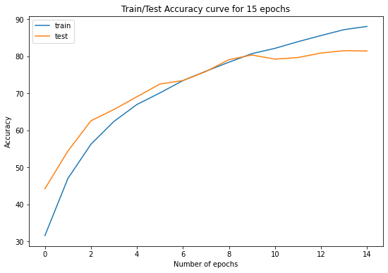
print(f"Average test Accuracy over {end_apochs} epochs: {sum(test_accuracy)//len(test_accuracy)}")
print(f"best test accuraccy over {end_apochs} epochs: {max(test_accuracy)}")

Average test Accuracy over 15 epochs: 72.0
best test accuraccy over 15 epochs: 81.54000091552734

figureName = 'WithMixUp' # change figure name

plt.figure(figsize=(9, 6))
plt.plot(results['epoch'].values, train_accuracy, label='train')
plt.plot(results['epoch'].values, test_accuracy, label='test')
plt.xlabel('Number of epochs')
plt.ylabel('Accuracy')
plt.title(f'Train/Test Accuracy curve for {end_apochs} epochs')
plt.savefig(f'/content/results/{figureName}.png')
plt.legend()
plt.show()

../../_images/9998ddf25657925b2bebb85ece674b77131c059f6ac1e9008c068874d4fd3145.png