Tutorial 2: Learning Hyperparameters

Tutorial 2: Learning Hyperparameters#

Week 1, Day 2: Linear Deep Learning

By Neuromatch Academy

Content creators: Saeed Salehi, Andrew Saxe

Content reviewers: Polina Turishcheva, Antoine De Comite, Kelson Shilling-Scrivo

Content editors: Anoop Kulkarni

Production editors: Khalid Almubarak, Gagana B, Spiros Chavlis

Tutorial Objectives#

Training landscape
The effect of depth
Choosing a learning rate
Initialization matters

Setup#

This a GPU-Free tutorial!

Install and import feedback gadget#

# Imports
import time
import numpy as np
import matplotlib
import matplotlib.pyplot as plt

Figure settings#

Plotting functions#

Show code cell source Hide code cell source

# @title Plotting functions

def plot_x_y_(x_t_, y_t_, x_ev_, y_ev_, loss_log_, weight_log_):
  """
  Plot train data and test results

  Args:
  x_t_: np.ndarray
    Training dataset
  y_t_: np.ndarray
    Ground truth corresponding to training dataset
  x_ev_: np.ndarray
    Evaluation set
  y_ev_: np.ndarray
    ShallowNarrowNet predictions
  loss_log_: list
    Training loss records
  weight_log_: list
    Training weight records (evolution of weights)

  Returns:
    Nothing
  """
  plt.figure(figsize=(12, 4))
  plt.subplot(1, 3, 1)
  plt.scatter(x_t_, y_t_, c='r', label='training data')
  plt.plot(x_ev_, y_ev_, c='b', label='test results', linewidth=2)
  plt.xlabel('x')
  plt.ylabel('y')
  plt.legend()
  plt.subplot(1, 3, 2)
  plt.plot(loss_log_, c='r')
  plt.xlabel('epochs')
  plt.ylabel('mean squared error')
  plt.subplot(1, 3, 3)
  plt.plot(weight_log_)
  plt.xlabel('epochs')
  plt.ylabel('weights')
  plt.show()


def plot_vector_field(what, init_weights=None):
  """
  Helper function to plot vector fields

  Args:
    what: string
      If "all", plot vectors, trajectories and loss function
      If "vectors", plot vectors
      If "trajectory", plot trajectories
      If "loss", plot loss function

  Returns:
    Nothing
  """
  n_epochs=40
  lr=0.15
  x_pos = np.linspace(2.0, 0.5, 100, endpoint=True)
  y_pos = 1. / x_pos
  xx, yy = np.mgrid[-1.9:2.0:0.2, -1.9:2.0:0.2]
  zz = np.empty_like(xx)
  x, y = xx[:, 0], yy[0]

  x_temp, y_temp = gen_samples(10, 1.0, 0.0)

  cmap = matplotlib.cm.plasma
  plt.figure(figsize=(8, 7))
  ax = plt.gca()

  if what == 'all' or what == 'vectors':
    for i, a in enumerate(x):
      for j, b in enumerate(y):
        temp_model = ShallowNarrowLNN([a, b])
        da, db = temp_model.dloss_dw(x_temp, y_temp)
        zz[i, j] = temp_model.loss(temp_model.forward(x_temp), y_temp)
        scale = min(40 * np.sqrt(da**2 + db**2), 50)
        ax.quiver(a, b, - da, - db, scale=scale, color=cmap(np.sqrt(da**2 + db**2)))

  if what == 'all' or what == 'trajectory':
    if init_weights is None:
      for init_weights in [[0.5, -0.5], [0.55, -0.45], [-1.8, 1.7]]:
        temp_model = ShallowNarrowLNN(init_weights)
        _, temp_records = temp_model.train(x_temp, y_temp, lr, n_epochs)
        ax.scatter(temp_records[:, 0], temp_records[:, 1],
                    c=np.arange(len(temp_records)), cmap='Greys')
        ax.scatter(temp_records[0, 0], temp_records[0, 1], c='blue', zorder=9)
        ax.scatter(temp_records[-1, 0], temp_records[-1, 1], c='red', marker='X', s=100, zorder=9)
    else:
      temp_model = ShallowNarrowLNN(init_weights)
      _, temp_records = temp_model.train(x_temp, y_temp, lr, n_epochs)
      ax.scatter(temp_records[:, 0], temp_records[:, 1],
                  c=np.arange(len(temp_records)), cmap='Greys')
      ax.scatter(temp_records[0, 0], temp_records[0, 1], c='blue', zorder=9)
      ax.scatter(temp_records[-1, 0], temp_records[-1, 1], c='red', marker='X', s=100, zorder=9)

  if what == 'all' or what == 'loss':
    contplt = ax.contourf(x, y, np.log(zz+0.001), zorder=-1, cmap='coolwarm', levels=100)
    divider = make_axes_locatable(ax)
    cax = divider.append_axes("right", size="5%", pad=0.05)
    cbar = plt.colorbar(contplt, cax=cax)
    cbar.set_label('log (Loss)')

  ax.set_xlabel("$w_1$")
  ax.set_ylabel("$w_2$")
  ax.set_xlim(-1.9, 1.9)
  ax.set_ylim(-1.9, 1.9)

  plt.show()


def plot_loss_landscape():
  """
  Helper function to plot loss landscapes

  Args:
    None

  Returns:
    Nothing
  """
  x_temp, y_temp = gen_samples(10, 1.0, 0.0)

  xx, yy = np.mgrid[-1.9:2.0:0.2, -1.9:2.0:0.2]
  zz = np.empty_like(xx)
  x, y = xx[:, 0], yy[0]

  for i, a in enumerate(x):
    for j, b in enumerate(y):
      temp_model = ShallowNarrowLNN([a, b])
      zz[i, j] = temp_model.loss(temp_model.forward(x_temp), y_temp)

  temp_model = ShallowNarrowLNN([-1.8, 1.7])
  loss_rec_1, w_rec_1 = temp_model.train(x_temp, y_temp, 0.02, 240)

  temp_model = ShallowNarrowLNN([1.5, -1.5])
  loss_rec_2, w_rec_2 = temp_model.train(x_temp, y_temp, 0.02, 240)

  plt.figure(figsize=(12, 8))
  ax = plt.subplot(1, 1, 1, projection='3d')
  ax.plot_surface(xx, yy, np.log(zz+0.5), cmap='coolwarm', alpha=0.5)
  ax.scatter3D(w_rec_1[:, 0], w_rec_1[:, 1], np.log(loss_rec_1+0.5),
                c='k', s=50, zorder=9)
  ax.scatter3D(w_rec_2[:, 0], w_rec_2[:, 1], np.log(loss_rec_2+0.5),
                c='k', s=50, zorder=9)
  plt.axis("off")
  ax.view_init(45, 260)

  plt.show()


def depth_widget(depth):
  """
  Simulate parameter in widget
  exploring impact of depth on the training curve
  (loss evolution) of a deep but narrow neural network.

  Args:
    depth: int
      Specifies depth of network

  Returns:
    Nothing
  """
  if depth == 0:
    depth_lr_init_interplay(depth, 0.02, 0.9)
  else:
    depth_lr_init_interplay(depth, 0.01, 0.9)


def lr_widget(lr):
  """
  Simulate parameters in widget
  exploring impact of depth on the training curve
  (loss evolution) of a deep but narrow neural network.

  Args:
    lr: float
      Specifies learning rate within network

  Returns:
    Nothing
  """
  depth_lr_init_interplay(50, lr, 0.9)


def depth_lr_interplay(depth, lr):
  """
  Simulate parameters in widget
  exploring impact of depth on the training curve
  (loss evolution) of a deep but narrow neural network.

  Args:
    depth: int
      Specifies depth of network
    lr: float
      Specifies learning rate within network

  Returns:
    Nothing
  """
  depth_lr_init_interplay(depth, lr, 0.9)


def depth_lr_init_interplay(depth, lr, init_weights):
  """
  Simulate parameters in widget
  exploring impact of depth on the training curve
  (loss evolution) of a deep but narrow neural network.

  Args:
    depth: int
      Specifies depth of network
    lr: float
      Specifies learning rate within network
    init_weights: list
      Specifies initial weights of the network

  Returns:
    Nothing
  """
  n_epochs = 600

  x_train, y_train = gen_samples(100, 2.0, 0.1)
  model = DeepNarrowLNN(np.full((1, depth+1), init_weights))

  plt.figure(figsize=(10, 5))
  plt.plot(model.train(x_train, y_train, lr, n_epochs),
            linewidth=3.0, c='m')

  plt.title("Training a {}-layer LNN with"
  " $\eta=${} initialized with $w_i=${}".format(depth, lr, init_weights), pad=15)
  plt.yscale('log')
  plt.xlabel('epochs')
  plt.ylabel('Log mean squared error')
  plt.ylim(0.001, 1.0)
  plt.show()


def plot_init_effect():
  """
  Helper function to plot evolution of log mean
  squared error over epochs

  Args:
    None

  Returns:
    Nothing
  """
  depth = 15
  n_epochs = 250
  lr = 0.02

  x_train, y_train = gen_samples(100, 2.0, 0.1)

  plt.figure(figsize=(12, 6))
  for init_w in np.arange(0.7, 1.09, 0.05):
      model = DeepNarrowLNN(np.full((1, depth), init_w))
      plt.plot(model.train(x_train, y_train, lr, n_epochs),
              linewidth=3.0, label="initial weights {:.2f}".format(init_w))
  plt.title("Training a {}-layer narrow LNN with $\eta=${}".format(depth, lr), pad=15)
  plt.yscale('log')
  plt.xlabel('epochs')
  plt.ylabel('Log mean squared error')
  plt.legend(loc='lower left', ncol=4)
  plt.ylim(0.001, 1.0)
  plt.show()


class InterPlay:
  """
  Class specifying parameters for widget
  exploring relationship between the depth
  and optimal learning rate
  """

  def __init__(self):
    """
    Initialize parameters for InterPlay

    Args:
      None

    Returns:
      Nothing
    """
    self.lr = [None]
    self.depth = [None]
    self.success = [None]
    self.min_depth, self.max_depth = 5, 65
    self.depth_list = np.arange(10, 61, 10)
    self.i_depth = 0
    self.min_lr, self.max_lr = 0.001, 0.105
    self.n_epochs = 600
    self.x_train, self.y_train = gen_samples(100, 2.0, 0.1)
    self.converged = False
    self.button = None
    self.slider = None

  def train(self, lr, update=False, init_weights=0.9):
    """
    Train network associated with InterPlay

    Args:
      lr: float
        Specifies learning rate within network
      init_weights: float
        Specifies initial weights of the network [default: 0.9]
      update: boolean
        If true, show updates on widget

    Returns:
      Nothing
    """
    if update and self.converged and self.i_depth < len(self.depth_list):
      depth = self.depth_list[self.i_depth]
      self.plot(depth, lr)
      self.i_depth += 1
      self.lr.append(None)
      self.depth.append(None)
      self.success.append(None)
      self.converged = False
      self.slider.value = 0.005
      if self.i_depth < len(self.depth_list):
        self.button.value = False
        self.button.description = 'Explore!'
        self.button.disabled = True
        self.button.button_style = 'Danger'
      else:
        self.button.value = False
        self.button.button_style = ''
        self.button.disabled = True
        self.button.description = 'Done!'
      time.sleep(1.0)

    elif self.i_depth < len(self.depth_list):
      depth = self.depth_list[self.i_depth]
      # Additional assert: self.min_depth <= depth <= self.max_depth
      assert self.min_lr <= lr <= self.max_lr
      self.converged = False

      model = DeepNarrowLNN(np.full((1, depth), init_weights))
      self.losses = np.array(model.train(self.x_train, self.y_train, lr, self.n_epochs))
      if np.any(self.losses < 1e-2):
        success = np.argwhere(self.losses < 1e-2)[0][0]
        if np.all((self.losses[success:] < 1e-2)):
          self.converged = True
          self.success[-1] = success
          self.lr[-1] = lr
          self.depth[-1] = depth
          self.button.disabled = False
          self.button.button_style = 'Success'
          self.button.description = 'Register!'
        else:
          self.button.disabled = True
          self.button.button_style = 'Danger'
          self.button.description = 'Explore!'
      else:
        self.button.disabled = True
        self.button.button_style = 'Danger'
        self.button.description = 'Explore!'
      self.plot(depth, lr)

  def plot(self, depth, lr):
    """
    Plot following subplots:
    a. Log mean squared error vs Epochs
    b. Learning time vs Depth
    c. Optimal learning rate vs Depth

    Args:
      depth: int
        Specifies depth of network
      lr: float
        Specifies learning rate of network

    Returns:
      Nothing
    """
    fig = plt.figure(constrained_layout=False, figsize=(10, 8))
    gs = fig.add_gridspec(2, 2)
    ax1 = fig.add_subplot(gs[0, :])
    ax2 = fig.add_subplot(gs[1, 0])
    ax3 = fig.add_subplot(gs[1, 1])

    ax1.plot(self.losses, linewidth=3.0, c='m')
    ax1.set_title("Training a {}-layer LNN with"
    " $\eta=${}".format(depth, lr), pad=15, fontsize=16)
    ax1.set_yscale('log')
    ax1.set_xlabel('epochs')
    ax1.set_ylabel('Log mean squared error')
    ax1.set_ylim(0.001, 1.0)

    ax2.set_xlim(self.min_depth, self.max_depth)
    ax2.set_ylim(-10, self.n_epochs)
    ax2.set_xlabel('Depth')
    ax2.set_ylabel('Learning time (Epochs)')
    ax2.set_title("Learning time vs depth", fontsize=14)
    ax2.scatter(np.array(self.depth), np.array(self.success), c='r')

    ax3.set_xlim(self.min_depth, self.max_depth)
    ax3.set_ylim(self.min_lr, self.max_lr)
    ax3.set_xlabel('Depth')
    ax3.set_ylabel('Optimal learning rate')
    ax3.set_title("Empirically optimal $\eta$ vs depth", fontsize=14)
    ax3.scatter(np.array(self.depth), np.array(self.lr), c='r')

    plt.show()

Helper functions#

Show code cell source Hide code cell source

# @title Helper functions

def gen_samples(n, a, sigma):
  """
  Generates n samples with
  `y = z * x + noise(sigma)` linear relation.

  Args:
    n : int
      Number of datapoints within sample
    a : float
      Offset of x
    sigma : float
      Standard deviation of distribution

  Returns:
    x : np.array
      if sigma > 0, x = random values
      else, x = evenly spaced numbers over a specified interval.
    y : np.array
      y = z * x + noise(sigma)
  """
  assert n > 0
  assert sigma >= 0

  if sigma > 0:
    x = np.random.rand(n)
    noise = np.random.normal(scale=sigma, size=(n))
    y = a * x + noise
  else:
    x = np.linspace(0.0, 1.0, n, endpoint=True)
    y = a * x
  return x, y


class ShallowNarrowLNN:
  """
  Shallow and narrow (one neuron per layer)
  linear neural network
  """

  def __init__(self, init_ws):
    """
    Initialize parameters of ShallowNarrowLNN

    Args:
      init_ws: initial weights as a list

    Returns:
      Nothing
    """
    assert isinstance(init_ws, list)
    assert len(init_ws) == 2
    self.w1 = init_ws[0]
    self.w2 = init_ws[1]

  def forward(self, x):
    """
    The forward pass through network y = x * w1 * w2

    Args:
      x: np.ndarray
        Input data

    Returns:
      y: np.ndarray
        y = x * w1 * w2
    """
    y = x * self.w1 * self.w2
    return y

  def loss(self, y_p, y_t):
    """
    Mean squared error (L2)
    with 1/2 for convenience

    Args:
      y_p: np.ndarray
        Network Predictions
      y_t: np.ndarray
        Targets

    Returns:
      mse: float
        Average mean squared error
    """
    assert y_p.shape == y_t.shape
    mse = ((y_t - y_p)**2).mean()
    return mse

  def dloss_dw(self, x, y_t):
    """
    Partial derivative of loss with respect to weights

    Args:
      x : np.array
        Input Dataset
      y_t : np.array
        Corresponding Ground Truth

    Returns:
      dloss_dw1: float
        -mean(2 * self.w2 * x * Error)
      dloss_dw2: float
        -mean(2 * self.w1 * x * Error)
    """
    assert x.shape == y_t.shape
    Error = y_t - self.w1 * self.w2 * x
    dloss_dw1 = - (2 * self.w2 * x * Error).mean()
    dloss_dw2 = - (2 * self.w1 * x * Error).mean()
    return dloss_dw1, dloss_dw2

  def train(self, x, y_t, eta, n_ep):
    """
    Gradient descent algorithm

    Args:
      x : np.array
        Input Dataset
      y_t : np.array
        Corrsponding target
      eta: float
        Learning rate
      n_ep : int
        Number of epochs

    Returns:
      loss_records: np.ndarray
        Log of loss per epoch
      weight_records: np.ndarray
        Log of weights per epoch
    """
    assert x.shape == y_t.shape

    loss_records = np.empty(n_ep)  # Pre allocation of loss records
    weight_records = np.empty((n_ep, 2))  # Pre allocation of weight records

    for i in range(n_ep):
      y_p = self.forward(x)
      loss_records[i] = self.loss(y_p, y_t)
      dloss_dw1, dloss_dw2 = self.dloss_dw(x, y_t)
      self.w1 -= eta * dloss_dw1
      self.w2 -= eta * dloss_dw2
      weight_records[i] = [self.w1, self.w2]

    return loss_records, weight_records


class DeepNarrowLNN:
  """
  Deep but thin (one neuron per layer)
  linear neural network
  """

  def __init__(self, init_ws):
    """
    Initialize parameters of DeepNarrowLNN

    Args:
      init_ws: np.ndarray
        Initial weights as a numpy array

    Returns:
      Nothing
    """
    self.n = init_ws.size
    self.W = init_ws.reshape(1, -1)

  def forward(self, x):
    """
    Forward pass of DeepNarrowLNN

    Args:
      x : np.array
        Input features

    Returns:
      y: np.array
        Product of weights over input features
    """
    y = np.prod(self.W) * x
    return y

  def loss(self, y_t, y_p):
    """
    Mean squared error (L2 loss)

    Args:
      y_t : np.array
        Targets
      y_p : np.array
        Network's predictions

    Returns:
      mse: float
        Mean squared error
    """
    assert y_p.shape == y_t.shape
    mse = ((y_t - y_p)**2 / 2).mean()
    return mse

  def dloss_dw(self, x, y_t, y_p):
    """
    Analytical gradient of weights

    Args:
      x : np.array
        Input features
      y_t : np.array
        Targets
      y_p : np.array
        Network Predictions

    Returns:
      dW: np.ndarray
        Analytical gradient of weights
    """
    E = y_t - y_p  # i.e., y_t - x * np.prod(self.W)
    Ex = np.multiply(x, E).mean()
    Wp = np.prod(self.W) / (self.W + 1e-9)
    dW = - Ex * Wp
    return dW

  def train(self, x, y_t, eta, n_epochs):
    """
    Training using gradient descent

    Args:
      x : np.array
        Input Features
      y_t : np.array
        Targets
      eta: float
        Learning rate
      n_epochs : int
        Number of epochs

    Returns:
      loss_records: np.ndarray
        Log of loss over epochs
    """
    loss_records = np.empty(n_epochs)
    loss_records[:] = np.nan
    for i in range(n_epochs):
      y_p = self.forward(x)
      loss_records[i] = self.loss(y_t, y_p).mean()
      dloss_dw = self.dloss_dw(x, y_t, y_p)
      if np.isnan(dloss_dw).any() or np.isinf(dloss_dw).any():
        return loss_records
      self.W -= eta * dloss_dw
    return loss_records

Set random seed#

Executing set_seed(seed=seed) you are setting the seed

Set device (GPU or CPU). Execute `set_device()`#

SEED = 2021
set_seed(seed=SEED)
DEVICE = set_device()

Random seed 2021 has been set.
GPU is not enabled in this notebook. 
If you want to enable it, in the menu under `Runtime` -> 
`Hardware accelerator.` and select `GPU` from the dropdown menu

Section 1: A Shallow Narrow Linear Neural Network#

Time estimate: ~30 mins

Video 1: Shallow Narrow Linear Net#

Submit your feedback#

Section 1.1: A Shallow Narrow Linear Net#

To better understand the behavior of neural network training with gradient descent, we start with the incredibly simple case of a shallow narrow linear neural net, since state-of-the-art models are impossible to dissect and comprehend with our current mathematical tools.

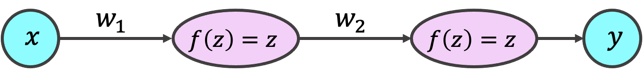
The model we use has one hidden layer, with only one neuron, and two weights. We consider the squared error (or L2 loss) as the cost function. As you may have already guessed, we can visualize the model as a neural network:

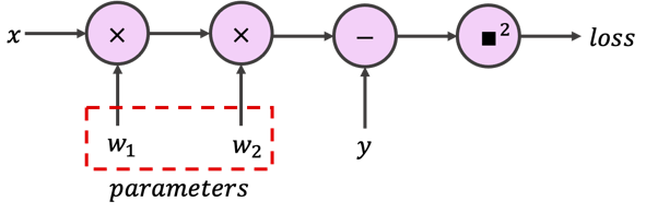
or by its computation graph:

or on a rare occasion, even as a reasonably compact mapping:

\[ loss = (y - w_1 \cdot w_2 \cdot x)^2 \]

Implementing a neural network from scratch without using any Automatic Differentiation tool is rarely necessary. The following two exercises are therefore Bonus (optional) exercises. Please ignore them if you have any time-limits or pressure and continue to Section 1.2.

Analytical Exercise 1.1: Loss Gradients (Optional)#

Once again, we ask you to calculate the network gradients analytically, since you will need them for the next exercise. We understand how annoying this is.

\(\dfrac{\partial{loss}}{\partial{w_1}} = ?\)

\(\dfrac{\partial{loss}}{\partial{w_2}} = ?\)

Solution#

\(\dfrac{\partial{loss}}{\partial{w_1}} = -2 \cdot w_2 \cdot x \cdot (y - w_1 \cdot w_2 \cdot x)\)

\(\dfrac{\partial{loss}}{\partial{w_2}} = -2 \cdot w_1 \cdot x \cdot (y - w_1 \cdot w_2 \cdot x)\)

Submit your feedback#

Coding Exercise 1.1: Implement simple narrow LNN (Optional)#

Next, we ask you to implement the forward pass for our model from scratch without using PyTorch.

Also, although our model gets a single input feature and outputs a single prediction, we could calculate the loss and perform training for multiple samples at once. This is the common practice for neural networks, since computers are incredibly fast doing matrix (or tensor) operations on batches of data, rather than processing samples one at a time through for loops. Therefore, for the loss function, please implement the mean squared error (MSE), and adjust your analytical gradients accordingly when implementing the dloss_dw function.

Finally, complete the train function for the gradient descent algorithm:

(20)#\[\begin{equation} \mathbf{w}^{(t+1)} = \mathbf{w}^{(t)} - \eta \nabla loss (\mathbf{w}^{(t)}) \end{equation}\]

class ShallowNarrowExercise:
  """
  Shallow and narrow (one neuron per layer) linear neural network
  """

  def __init__(self, init_weights):
    """
    Initialize parameters of ShallowNarrow Net

    Args:
      init_weights: list
        Initial weights

    Returns:
      Nothing
    """
    assert isinstance(init_weights, (list, np.ndarray, tuple))
    assert len(init_weights) == 2
    self.w1 = init_weights[0]
    self.w2 = init_weights[1]


  def forward(self, x):
    """
    The forward pass through netwrok y = x * w1 * w2

    Args:
      x: np.ndarray
        Features (inputs) to neural net

    Returns:
      y: np.ndarray
        Neural network output (predictions)
    """
    #################################################
    ## Implement the forward pass to calculate prediction
    ## Note that prediction is not the loss
    # Complete the function and remove or comment the line below
    raise NotImplementedError("Forward Pass `forward`")
    #################################################
    y = ...
    return y


  def dloss_dw(self, x, y_true):
    """
    Gradient of loss with respect to weights

    Args:
      x: np.ndarray
        Features (inputs) to neural net
      y_true: np.ndarray
        True labels

    Returns:
      dloss_dw1: float
        Mean gradient of loss with respect to w1
      dloss_dw2: float
        Mean gradient of loss with respect to w2
    """
    assert x.shape == y_true.shape
    #################################################
    ## Implement the gradient computation function
    # Complete the function and remove or comment the line below
    raise NotImplementedError("Gradient of Loss `dloss_dw`")
    #################################################
    dloss_dw1 = ...
    dloss_dw2 = ...
    return dloss_dw1, dloss_dw2


  def train(self, x, y_true, lr, n_ep):
    """
    Training with Gradient descent algorithm

    Args:
      x: np.ndarray
        Features (inputs) to neural net
      y_true: np.ndarray
        True labels
      lr: float
        Learning rate
      n_ep: int
        Number of epochs (training iterations)

    Returns:
      loss_records: list
        Training loss records
      weight_records: list
        Training weight records (evolution of weights)
    """
    assert x.shape == y_true.shape

    loss_records = np.empty(n_ep)  # Pre allocation of loss records
    weight_records = np.empty((n_ep, 2))  # Pre allocation of weight records

    for i in range(n_ep):
      y_prediction = self.forward(x)
      loss_records[i] = loss(y_prediction, y_true)
      dloss_dw1, dloss_dw2 = self.dloss_dw(x, y_true)
      #################################################
      ## Implement the gradient descent step
      # Complete the function and remove or comment the line below
      raise NotImplementedError("Training loop `train`")
      #################################################
      self.w1 -= ...
      self.w2 -= ...
      weight_records[i] = [self.w1, self.w2]

    return loss_records, weight_records


def loss(y_prediction, y_true):
  """
  Mean squared error

  Args:
    y_prediction: np.ndarray
      Model output (prediction)
    y_true: np.ndarray
      True label

  Returns:
    mse: np.ndarray
      Mean squared error loss
  """
  assert y_prediction.shape == y_true.shape
  #################################################
  ## Implement the MEAN squared error
  # Complete the function and remove or comment the line below
  raise NotImplementedError("Loss function `loss`")
  #################################################
  mse = ...
  return mse



set_seed(seed=SEED)
n_epochs = 211
learning_rate = 0.02
initial_weights = [1.4, -1.6]
x_train, y_train = gen_samples(n=73, a=2.0, sigma=0.2)
x_eval = np.linspace(0.0, 1.0, 37, endpoint=True)
## Uncomment to run
# sn_model = ShallowNarrowExercise(initial_weights)
# loss_log, weight_log = sn_model.train(x_train, y_train, learning_rate, n_epochs)
# y_eval = sn_model.forward(x_eval)
# plot_x_y_(x_train, y_train, x_eval, y_eval, loss_log, weight_log)

Random seed 2021 has been set.

Click for solution

Submit your feedback#

Section 1.2: Learning landscapes#

Video 2: Training Landscape#

Submit your feedback#

As you may have already asked yourself, we can analytically find \(w_1\) and \(w_2\) without using gradient descent:

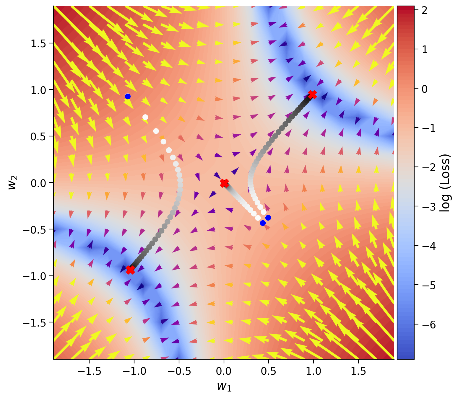
(21)#\[\begin{equation} w_1 \cdot w_2 = \dfrac{y}{x} \end{equation}\]

In fact, we can plot the gradients, the loss function and all the possible solutions in one figure. In this example, we use the \(y = 1x\) mapping:

Blue ribbon: shows all possible solutions: \(~ w_1 w_2 = \dfrac{y}{x} = \dfrac{x}{x} = 1 \Rightarrow w_1 = \dfrac{1}{w_2}\)

Contour background: Shows the loss values, red being higher loss

Vector field (arrows): shows the gradient vector field. The larger yellow arrows show larger gradients, which correspond to bigger steps by gradient descent.

Scatter circles: the trajectory (evolution) of weights during training for three different initializations, with blue dots marking the start of training and red crosses ( x ) marking the end of training. You can also try your own initializations (keep the initial values between -2.0 and 2.0) as shown here:

plot_vector_field('all', [1.0, -1.0])

Finally, if the plot is too crowded, feel free to pass one of the following strings as argument:

plot_vector_field('vectors')  # For vector field
plot_vector_field('trajectory')  # For training trajectory
plot_vector_field('loss')  # For loss contour

Think!

Explore the next two plots. Try different initial values. Can you find the saddle point? Why does training slow down near the minima?

plot_vector_field('all')

../../../_images/b2c72bebca4f83cb4f4eaf6f8abd90f6e9200fbfb1d2b4c301ce441b41803f8a.png

Here, we also visualize the loss landscape in a 3-D plot, with two training trajectories for different initial conditions. Note: the trajectories from the 3D plot and the previous plot are independent and different.

plot_loss_landscape()

../../../_images/a929da8da1b2ef2bcf7555e64b02623d058e275714fc2799073034aa8b006012.png

Video 3: Training Landscape - Discussion#

Submit your feedback#

Section 2: Depth, Learning rate, and initialization#

Time estimate: ~45 mins

Successful deep learning models are often developed by a team of very clever people, spending many many hours “tuning” learning hyperparameters, and finding effective initializations. In this section, we look at three basic (but often not simple) hyperparameters: depth, learning rate, and initialization.

Section 2.1: The effect of depth#

Video 4: Effect of Depth#

Submit your feedback#

Why might depth be useful? What makes a network or learning system “deep”? The reality is that shallow neural nets are often incapable of learning complex functions due to data limitations. On the other hand, depth seems like magic. Depth can change the functions a network can represent, the way a network learns, and how a network generalizes to unseen data.

So let’s look at the challenges that depth poses in training a neural network. Imagine a single input, single output linear network with 50 hidden layers and only one neuron per layer (i.e. a narrow deep neural network). The output of the network is easy to calculate:

\[ prediction = x \cdot w_1 \cdot w_2 \cdot \cdot \cdot w_{50} \]

If the initial value for all the weights is \(w_i = 2\), the prediction for \(x=1\) would be exploding: \(y_p = 2^{50} \approx 1.1256 \times 10^{15}\). On the other hand, for weights initialized to \(w_i = 0.5\), the output is vanishing: \(y_p = 0.5^{50} \approx 8.88 \times 10^{-16}\). Similarly, if we recall the chain rule, as the graph gets deeper, the number of elements in the chain multiplication increases, which could lead to exploding or vanishing gradients. To avoid such numerical vulnerablities that could impair our training algorithm, we need to understand the effect of depth.

Interactive Demo 2.1: Depth widget#

Use the widget to explore the impact of depth on the training curve (loss evolution) of a deep but narrow neural network.

Think!

Which networks trained the fastest? Did all networks eventually “work” (converge)? What is the shape of their learning trajectory?

Make sure you execute this cell to enable the widget!

Video 5: Effect of Depth - Discussion#

Submit your feedback#

Section 2.2: Choosing a learning rate#

The learning rate is a common hyperparameter for most optimization algorithms. How should we set it? Sometimes the only option is to try all the possibilities, but sometimes knowing some key trade-offs will help guide our search for good hyperparameters.

Video 6: Learning Rate#

Submit your feedback#

Interactive Demo 2.2: Learning rate widget#

Here, we fix the network depth to 50 layers. Use the widget to explore the impact of learning rate \(\eta\) on the training curve (loss evolution) of a deep but narrow neural network.

Think!

Can we say that larger learning rates always lead to faster learning? Why not?

Make sure you execute this cell to enable the widget!

Video 7: Learning Rate - Discussion#

Submit your feedback#

Section 2.3: Depth vs Learning Rate#

Video 8: Depth and Learning Rate#

Submit your feedback#

Interactive Demo 2.3: Depth and Learning Rate#

Important instruction The exercise starts with 10 hidden layers. Your task is to find the learning rate that delivers fast but robust convergence (learning). When you are confident about the learning rate, you can Register the optimal learning rate for the given depth. Once you press register, a deeper model is instantiated, so you can find the next optimal learning rate. The Register button turns green only when the training converges, but does not imply the fastest convergence. Finally, be patient :) the widgets are slow.

Think!

Can you explain the relationship between the depth and optimal learning rate?

Make sure you execute this cell to enable the widget!

Submit your feedback#

Video 9: Depth and Learning Rate - Discussion#

Submit your feedback#

Section 2.4: Why initialization is important#

Video 10: Initialization Matters#

Submit your feedback#

We’ve seen, even in the simplest of cases, that depth can slow learning. Why? From the chain rule, gradients are multiplied by the current weight at each layer, so the product can vanish or explode. Therefore, weight initialization is a fundamentally important hyperparameter.

Although in practice initial values for learnable parameters are often sampled from different \(\mathcal{Uniform}\) or \(\mathcal{Normal}\) probability distribution, here we use a single value for all the parameters.

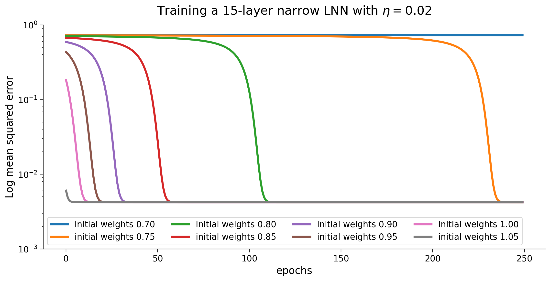
The figure below shows the effect of initialization on the speed of learning for the deep but narrow LNN. We have excluded initializations that lead to numerical errors such as nan or inf, which are the consequence of smaller or larger initializations.

Make sure you execute this cell to see the figure!

../../../_images/d50b0bb5be799a5938cc05673941c07c15ae6d4203f35bc93551e6831ce2318c.png

Video 11: Initialization Matters - Discussion#

Submit your feedback#

Summary#

In the second tutorial, we have learned what is the training landscape, and also we have see in depth the effect of the depth of the network and the learning rate, and their interplay. Finally, we have seen that initialization matters and why we need smart ways of initialization.

Video 12: Tutorial 2 Wrap-up#

Submit your feedback#

Bonus#

Hyperparameter interaction#

Finally, let’s put everything we learned together and find best initial weights and learning rate for a given depth. By now you should have learned the interactions and know how to find the optimal values quickly. If you get numerical overflow warnings, don’t be discouraged! They are often caused by “exploding” or “vanishing” gradients.

Think!

Did you experience any surprising behaviour or difficulty finding the optimal parameters?

Make sure you execute this cell to enable the widget!

Tutorial 2: Learning Hyperparameters

Contents

Tutorial 2: Learning Hyperparameters#

Tutorial Objectives#

Setup#

Install and import feedback gadget#

Figure settings#

Plotting functions#

Helper functions#

Set random seed#

Set device (GPU or CPU). Execute set_device()#

Section 1: A Shallow Narrow Linear Neural Network#

Video 1: Shallow Narrow Linear Net#

Submit your feedback#

Section 1.1: A Shallow Narrow Linear Net#

Analytical Exercise 1.1: Loss Gradients (Optional)#

Solution#

Submit your feedback#

Coding Exercise 1.1: Implement simple narrow LNN (Optional)#

Submit your feedback#

Section 1.2: Learning landscapes#

Video 2: Training Landscape#

Submit your feedback#

Video 3: Training Landscape - Discussion#

Submit your feedback#

Section 2: Depth, Learning rate, and initialization#

Section 2.1: The effect of depth#

Video 4: Effect of Depth#

Submit your feedback#

Interactive Demo 2.1: Depth widget#

Video 5: Effect of Depth - Discussion#

Submit your feedback#

Section 2.2: Choosing a learning rate#

Video 6: Learning Rate#

Submit your feedback#

Interactive Demo 2.2: Learning rate widget#

Video 7: Learning Rate - Discussion#

Submit your feedback#

Section 2.3: Depth vs Learning Rate#

Video 8: Depth and Learning Rate#

Submit your feedback#

Interactive Demo 2.3: Depth and Learning Rate#

Submit your feedback#

Video 9: Depth and Learning Rate - Discussion#

Submit your feedback#

Section 2.4: Why initialization is important#

Video 10: Initialization Matters#

Submit your feedback#

Video 11: Initialization Matters - Discussion#

Submit your feedback#

Summary#

Video 12: Tutorial 2 Wrap-up#

Submit your feedback#

Bonus#

Hyperparameter interaction#

Submit your feedback#

Set device (GPU or CPU). Execute `set_device()`#