Tutorial 1: Regularization techniques part 1

Tutorial 1: Regularization techniques part 1#

Week 2, Day 1: Regularization

By Neuromatch Academy

Content creators: Ravi Teja Konkimalla, Mohitrajhu Lingan Kumaraian, Kevin Machado Gamboa, Kelson Shilling-Scrivo, Lyle Ungar

Content reviewers: Piyush Chauhan, Siwei Bai, Kelson Shilling-Scrivo

Content editors: Roberto Guidotti, Spiros Chavlis

Production editors: Saeed Salehi, Gagana B, Spiros Chavlis

Tutorial Objectives#

Big Artificial Neural Networks (ANNs) are efficient universal approximators due to their adaptive basis functions
ANNs memorize some but generalize well
Regularization as shrinkage of overparameterized models: early stopping

Setup#

Note that some of the code for today can take up to an hour to run. We have therefore “hidden” the code and shown the resulting outputs.

Install dependencies#

WARNING: There may be errors and/or warnings reported during the installation. However, they should be ignored.

Install and import feedback gadget#

# Imports
import time
import copy
import torch
import pathlib

import numpy as np
import torch.nn as nn
import torch.optim as optim
import torch.nn.functional as F
import matplotlib.pyplot as plt
import matplotlib.animation as animation

from tqdm.auto import tqdm
from IPython.display import HTML
from torchvision import transforms
from torchvision.datasets import ImageFolder

Figure Settings#

Loading Animal Faces data#

Start downloading and unzipping `AnimalFaces` dataset...

Download completed.

Loading Animal Faces Randomized data#

Start downloading and unzipping `Randomized AnimalFaces` dataset...

Download completed.

Plotting functions#

Set random seed#

Executing set_seed(seed=seed) you are setting the seed

Set device (GPU or CPU). Execute `set_device()`#

SEED = 2021
set_seed(seed=SEED)
DEVICE = set_device()

Random seed 2021 has been set.
WARNING: For this notebook to perform best, if possible, in the menu under `Runtime` -> `Change runtime type.`  select `GPU` 

Section 0: Defining useful functions#

Let’s start the tutorial by defining some functions which we will use frequently today, such as: AnimalNet, train, test and main.

class AnimalNet(nn.Module):
  """
  Network Class - Animal Faces
  """

  def __init__(self):
    """
    Initialize parameters of AnimalNet

    Args:
      None

    Returns:
      Nothing
    """
    super(AnimalNet, self).__init__()
    self.fc1 = nn.Linear(3 * 32 * 32, 128)
    self.fc2 = nn.Linear(128, 32)
    self.fc3 = nn.Linear(32, 3)

  def forward(self, x):
    """
    Forward Pass of AnimalNet

    Args:
      x: torch.tensor
        Input features

    Returns:
      output: torch.tensor
        Outputs/Predictions
    """
    x = x.view(x.shape[0],-1)
    x = F.relu(self.fc1(x))
    x = F.relu(self.fc2(x))
    x = self.fc3(x)
    output = F.log_softmax(x, dim=1)
    return output

The train function takes in the current model, along with the train_loader and loss function, and updates the parameters for a single pass of the entire dataset. The test function takes in the current model after every epoch and calculates the accuracy on the test dataset.

def train(args, model, train_loader, optimizer,
          reg_function1=None, reg_function2=None, criterion=F.nll_loss):
  """
  Trains the current input model using the data
  from Train_loader and Updates parameters for a single pass

  Args:
    args: dictionary
      Dictionary with epochs: 200, lr: 5e-3, momentum: 0.9, device: DEVICE
    model: nn.module
      Neural network instance
    train_loader: torch.loader
      Input dataset
    optimizer: function
      Optimizer
    reg_function1: function
      Regularisation function [default: None]
    reg_function2: function
      Regularisation function [default: None]
    criterion: function
      Specifies loss function [default: nll_loss]

  Returns:
    model: nn.module
      Neural network instance post training
  """
  device = args['device']
  model.train()
  for batch_idx, (data, target) in enumerate(train_loader):
    data, target = data.to(device), target.to(device)
    optimizer.zero_grad()
    output = model(data)
    if reg_function1 is None:
      loss = criterion(output, target)
    elif reg_function2 is None:
      loss = criterion(output, target)+args['lambda']*reg_function1(model)
    else:
      loss = criterion(output, target) + args['lambda1']*reg_function1(model) + args['lambda2']*reg_function2(model)
    loss.backward()
    optimizer.step()

  return model


def test(model, test_loader, criterion=F.nll_loss, device='cpu'):
  """
  Tests the current model

  Args:
    model: nn.module
      Neural network instance
    device: string
      GPU/CUDA if available, CPU otherwise
    test_loader: torch.loader
      Test dataset
    criterion: function
      Specifies loss function [default: nll_loss]

  Returns:
    test_loss: float
      Test loss
  """
  model.eval()
  test_loss = 0
  correct = 0
  with torch.no_grad():
    for data, target in test_loader:
      data, target = data.to(device), target.to(device)
      output = model(data)
      test_loss += criterion(output, target, reduction='sum').item()  # Sum up batch loss
      pred = output.argmax(dim=1, keepdim=True)  # Get the index of the max log-probability
      correct += pred.eq(target.view_as(pred)).sum().item()

  test_loss /= len(test_loader.dataset)
  return 100. * correct / len(test_loader.dataset)


def main(args, model, train_loader, val_loader,
         reg_function1=None, reg_function2=None):
  """
  Trains the model with train_loader and
  tests the learned model using val_loader

  Args:
    args: dictionary
      Dictionary with epochs: 200, lr: 5e-3, momentum: 0.9, device: DEVICE
    model: nn.module
      Neural network instance
    train_loader: torch.loader
      Train dataset
    val_loader: torch.loader
      Validation set
    reg_function1: function
      Regularisation function [default: None]
    reg_function2: function
      Regularisation function [default: None]

  Returns:
    val_acc_list: list
      Log of validation accuracy
    train_acc_list: list
      Log of training accuracy
    param_norm_list: list
      Log of frobenius norm
    trained_model: nn.module
      Trained model/model post training
  """

  device = args['device']

  model = model.to(device)
  optimizer = optim.SGD(model.parameters(), lr=args['lr'],
                        momentum=args['momentum'])

  val_acc_list, train_acc_list,param_norm_list = [], [], []
  for epoch in tqdm(range(args['epochs'])):
    trained_model = train(args, model, train_loader, optimizer,
                          reg_function1=reg_function1,
                          reg_function2=reg_function2)
    train_acc = test(trained_model, train_loader, device=device)
    val_acc = test(trained_model, val_loader, device=device)
    param_norm = calculate_frobenius_norm(trained_model)
    train_acc_list.append(train_acc)
    val_acc_list.append(val_acc)
    param_norm_list.append(param_norm)

  return val_acc_list, train_acc_list, param_norm_list, trained_model

Section 1: Regularization is Shrinkage#

Time estimate: ~20 mins

Video 1: Introduction to Regularization#

Submit your feedback#

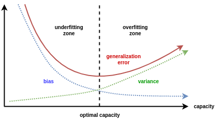
A key idea of neural nets is that they use models that are “too complex” - complex enough to fit all the noise in the data. One then needs to “regularize” them to make the models fit complex enough, but not too complex. The more complex the model, the better it fits the training data, but if it is too complex, it generalizes less well; it memorizes the training data but is less accurate on future test data.

Video 2: Regularization as Shrinkage#

Submit your feedback#

One way to think about Regularization is to think in terms of the magnitude of the overall weights of the model. A model with big weights can fit more data perfectly, whereas a model with smaller weights tends to underperform on the train set but can surprisingly do very well on the test set. Having the weights too small can also be an issue as it can then underfit the model.

In these tutorials, we use the sum of the Frobenius norm of all the tensors in the model as a measure of the “size of the model”.

Coding Exercise 1: Frobenius Norm#

Before we start, let’s define the Frobenius norm, sometimes also called the Euclidean norm of an \(m×n\) matrix \(A\) as the square root of the sum of the absolute squares of its elements.

(57)#\[\begin{equation} ||A||_F= \sqrt{\sum_{i=1}^m\sum_{j=1}^n|a_{ij}|^2} \end{equation}\]

This is just a measure of how big the matrix is, analogous to how big a vector is.

Hint: Use the functions model.parameters() or model.named_parameters()

def calculate_frobenius_norm(model):
  """
  Function to calculate frobenius norm

  Args:
    model: nn.module
      Neural network instance

  Returns:
    norm: float
      Frobenius norm
  """
  ####################################################################
  # Fill in all missing code below (...),
  # then remove or comment the line below to test your function
  raise NotImplementedError("Define `calculate_frobenius_norm` function")
  ####################################################################
  norm = 0.0
  # Sum the square of all parameters
  for param in model.parameters():
    norm += ...

  # Take a square root of the sum of squares of all the parameters
  norm = ...
  return norm



# Seed added for reproducibility
set_seed(seed=SEED)

## uncomment below to test your code
# net = nn.Linear(10, 1)
# print(f'Frobenius norm of Single Linear Layer: {calculate_frobenius_norm(net)}')

Random seed 2021 has been set.

Random seed 2021 has been set.
Frobenius Norm of Single Linear Layer: 0.6572162508964539

Click for solution

Submit your feedback#

Apart from calculating the weight size for an entire model, we could also determine the weight size in every layer. For this, we can modify our calculate_frobenius_norm function as shown below.

Have a look how it works!!

def calculate_frobenius_norm(model):
  """
  Calculate Frobenius Norm per Layer

  Args:
    model: nn.module
      Neural network instance

  Returns:
    norm: float
      Norm value
    labels: list
      Targets
    ws: list
      Weights
  """

  # Initialization of variables
  norm, ws, labels = 0.0, [], []

  # Sum all the parameters
  for name, parameters in model.named_parameters():
    p = torch.sum(parameters**2)
    norm += p

    ws.append((p**0.5).cpu().detach().numpy())
    labels.append(name)

  # Take a square root of the sum of squares of all the parameters
  norm = (norm**0.5).cpu().detach().numpy()

  return norm, ws, labels


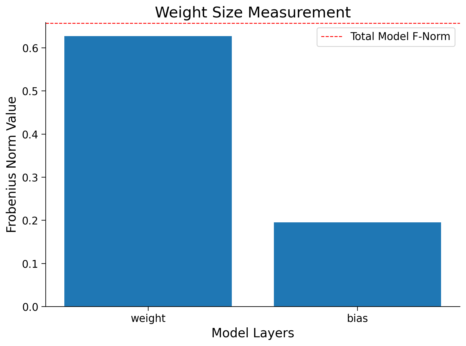
set_seed(SEED)
net = nn.Linear(10,1)
norm, ws, labels = calculate_frobenius_norm(net)
print(f'Frobenius norm of Single Linear Layer: {norm:.4f}')
# Plots the weights
plot_weights(norm, labels, ws)

Random seed 2021 has been set.
Frobenius norm of Single Linear Layer: 0.6572

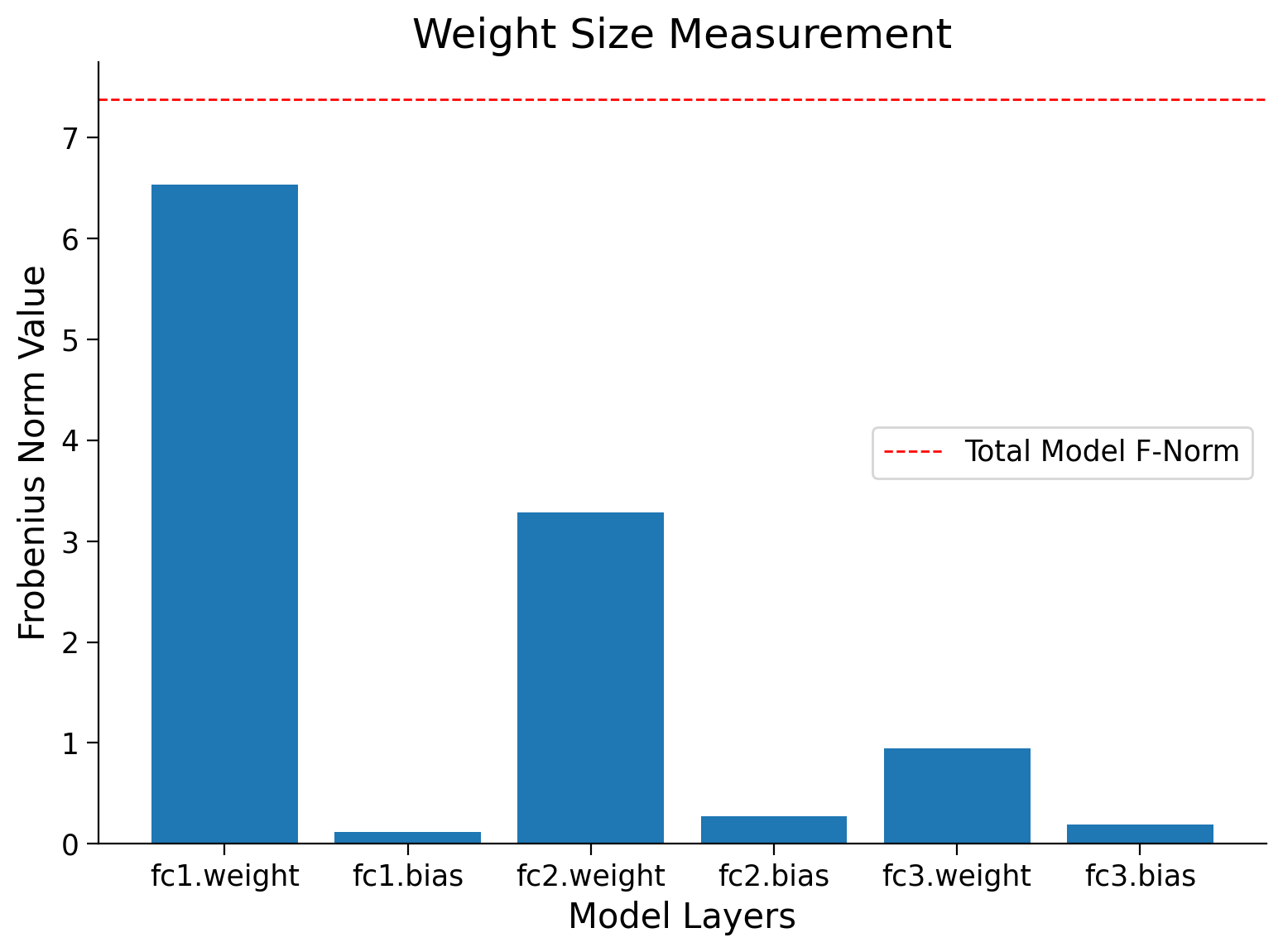
../../../_images/7f96db181f1246bf7033cc953839a1c263a55b81faf06b89209f8ed1237fcf00.png

Using the last function, calculate_frobenius_norm, we can also obtain the Frobenius norm per layer for a whole ANN model and use the plot_weigts function to visualize them.

set_seed(seed=SEED)

# Creates a new model
model = AnimalNet()

# Calculates the forbenius norm per layer
norm, ws, labels = calculate_frobenius_norm(model)
print(f'Frobenius norm of Models weights: {norm:.4f}')

# Plots the weights
plot_weights(norm, labels, ws)

Random seed 2021 has been set.
Frobenius norm of Models weights: 7.3810

../../../_images/c3d6f36997c074b0a8a6d31836859b54f631b834fd9bab539fc1c013a9b96c37.png

Section 2: Overfitting#

Time estimate: ~15 mins

Video 3: Overparameterization and Overfitting#

Submit your feedback#

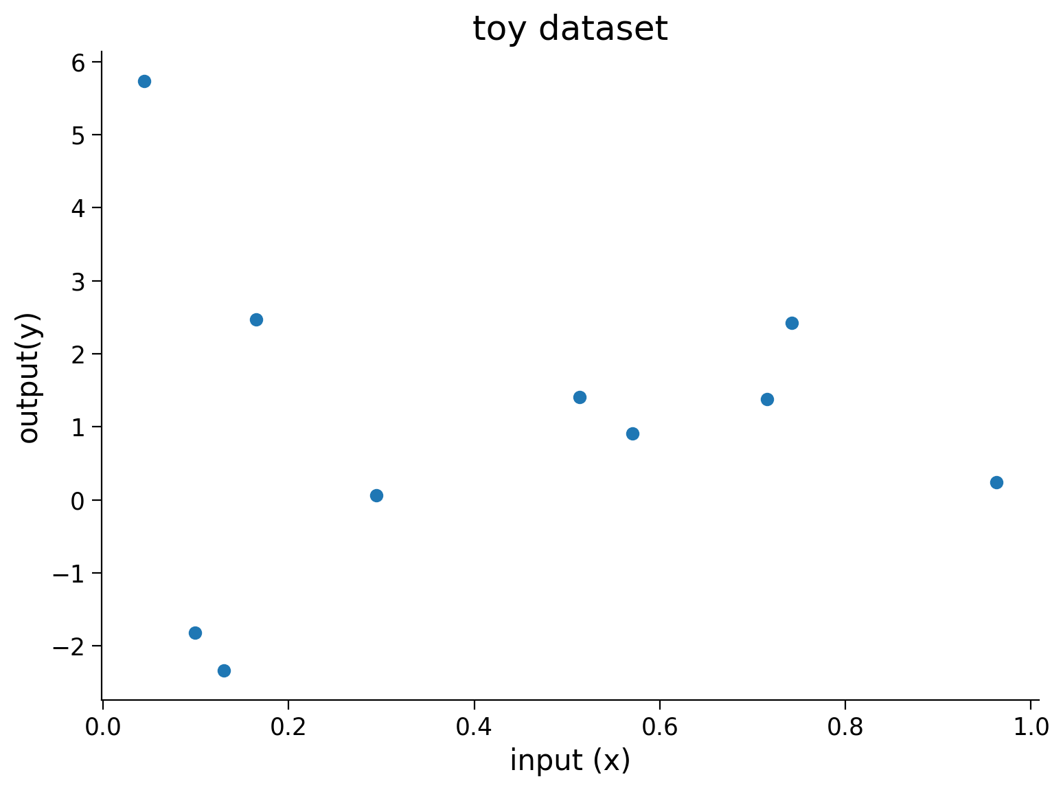
Section 2.1: Visualizing Overfitting#

Let’s create some synthetic dataset that we will use to illustrate overfitting in neural networks.

set_seed(seed=SEED)

# Creating train data
# Input
X = torch.rand((10, 1))
# Output
Y = 2*X + 2*torch.empty((X.shape[0], 1)).normal_(mean=0, std=1)  # Adding small error in the data

# Visualizing train data
plt.figure(figsize=(8, 6))
plt.scatter(X.numpy(),Y.numpy())
plt.xlabel('input (x)')
plt.ylabel('output(y)')
plt.title('toy dataset')
plt.show()

# Creating test dataset
X_test = torch.linspace(0, 1, 40)
X_test = X_test.reshape((40, 1, 1))

Random seed 2021 has been set.

../../../_images/0367ec8db8ae4d65ea628497d7d5f591ff01c92e4fc01ec7dad4cccfb52e97ba.png

Let’s create an overparametrized Neural Network that can fit on the dataset that we just created and train it.

First, let’s build the model architecture:

class Net(nn.Module):
  """
  Network Class - 2D with following structure
  nn.Linear(1, 300) + leaky_relu(self.fc1(x)) # First fully connected layer
  nn.Linear(300, 500) + leaky_relu(self.fc2(x)) # Second fully connected layer
  nn.Linear(500, 1) # Final fully connected layer
  """

  def __init__(self):
    """
    Initialize parameters of Net

    Args:
      None

    Returns:
      Nothing
    """
    super(Net, self).__init__()

    self.fc1 = nn.Linear(1, 300)
    self.fc2 = nn.Linear(300, 500)
    self.fc3 = nn.Linear(500, 1)

  def forward(self, x):
    """
    Forward pass of Net

    Args:
      x: torch.tensor
        Input features

    Returns:
      x: torch.tensor
        Output/Predictions
    """
    x = F.leaky_relu(self.fc1(x))
    x = F.leaky_relu(self.fc2(x))
    output = self.fc3(x)
    return output

Next, let’s define the different parameters for training our model:

set_seed(seed=SEED)

# Train the network on toy dataset
model = Net()

criterion = nn.MSELoss()
optimizer = optim.Adam(model.parameters(), lr=1e-4)

iters = 0
# Calculates frobenius before training
normi, wsi, label = calculate_frobenius_norm(model)

Random seed 2021 has been set.

At this point, we can now train our model.

set_seed(seed=SEED)

# Initializing variables
# Losses
train_loss = []
test_loss = []

# Model norm
model_norm = []

# Initializing variables to store weights
norm_per_layer = []

max_epochs = 10000

running_predictions = np.empty((40, int(max_epochs / 500 + 1)))

for epoch in tqdm(range(max_epochs)):
  # Frobenius norm per epoch
  norm, pl, layer_names = calculate_frobenius_norm(model)

  # Training
  model_norm.append(norm)
  norm_per_layer.append(pl)
  model.train()
  optimizer.zero_grad()
  predictions = model(X)
  loss = criterion(predictions, Y)
  loss.backward()
  optimizer.step()

  train_loss.append(loss.data)
  model.eval()
  Y_test = model(X_test)
  loss = criterion(Y_test, 2*X_test)
  test_loss.append(loss.data)

  if (epoch % 500 == 0 or epoch == max_epochs - 1):
    running_predictions[:, iters] = Y_test[:, 0, 0].detach().numpy()
    iters += 1

Random seed 2021 has been set.

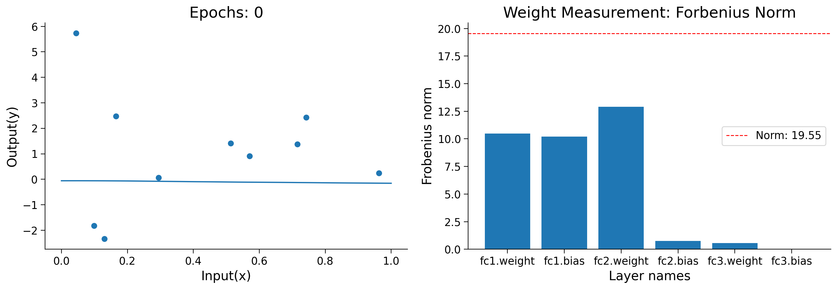
Now that we have finished training, let’s see how the model has evolved over the training process.

Animation (Run Me!)#

Random seed 2021 has been set.

---------------------------------------------------------------------------
RuntimeError                              Traceback (most recent call last)
Cell In[28], line 53
     47   return plot1, plot2
     50 anim = animation.FuncAnimation(fig, frame, frames=range(20),
     51                                blit=False, repeat=False,
     52                                repeat_delay=10000)
---> 53 html_anim = HTML(anim.to_html5_video())
     54 plt.close()
     56 import IPython

File /opt/hostedtoolcache/Python/3.9.19/x64/lib/python3.9/site-packages/matplotlib/animation.py:1285, in Animation.to_html5_video(self, embed_limit)
   1282 path = Path(tmpdir, "temp.m4v")
   1283 # We create a writer manually so that we can get the
   1284 # appropriate size for the tag
-> 1285 Writer = writers[mpl.rcParams['animation.writer']]
   1286 writer = Writer(codec='h264',
   1287                 bitrate=mpl.rcParams['animation.bitrate'],
   1288                 fps=1000. / self._interval)
   1289 self.save(str(path), writer=writer)

File /opt/hostedtoolcache/Python/3.9.19/x64/lib/python3.9/site-packages/matplotlib/animation.py:148, in MovieWriterRegistry.__getitem__(self, name)
    146 if self.is_available(name):
    147     return self._registered[name]
--> 148 raise RuntimeError(f"Requested MovieWriter ({name}) not available")

RuntimeError: Requested MovieWriter (ffmpeg) not available

../../../_images/66423f415c5ed2c155e6d4c8df35ddcaef422be800f1752e6da3c3185e7cab70.png

Plot the train and test losses#

../../../_images/a5d3cad3009c0a9f95bd70801d179e595c8bf2e6d474bcc0b05541d7407725f3.png

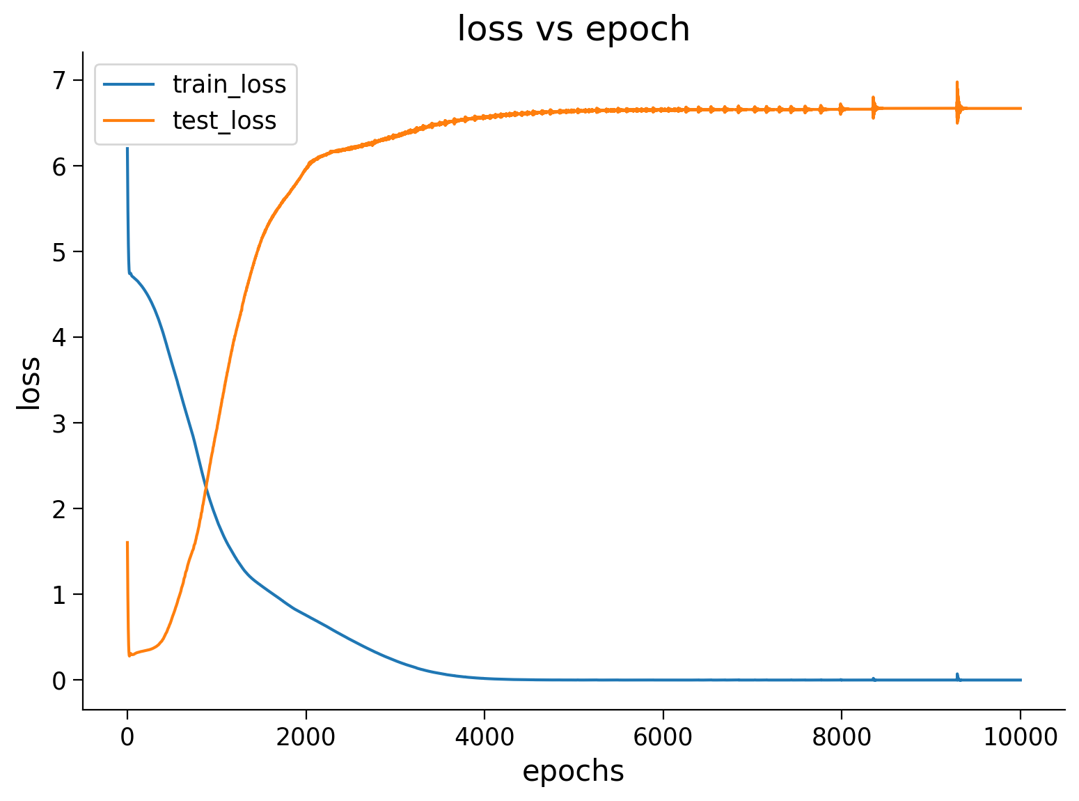
Think! 2.1: Interpreting losses#

Regarding the train and test graph above, discuss among yourselves:

What trend do you see with respect to train and test losses (Where do you see the minimum of these losses?)
What does it tell us about the model we trained?

Click for solution

Submit your feedback#

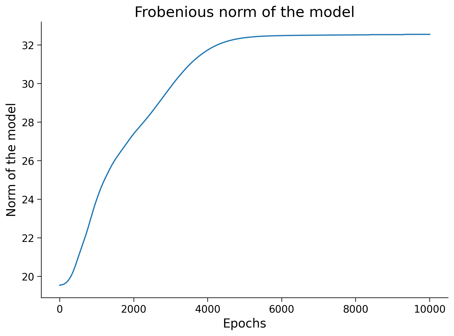
Now let’s visualize the Frobenious norm of the model as we trained. You should see that the value of weights increases over the epochs.

Frobenious norm of the model

../../../_images/9d2db9ca12067f24eff8013482b01d974c3ad921f256ab2cec85fa57d86e789d.png

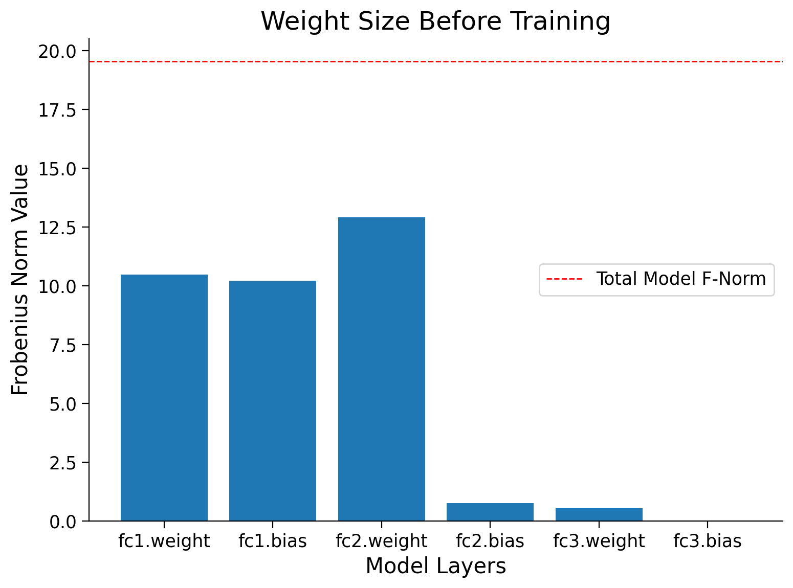
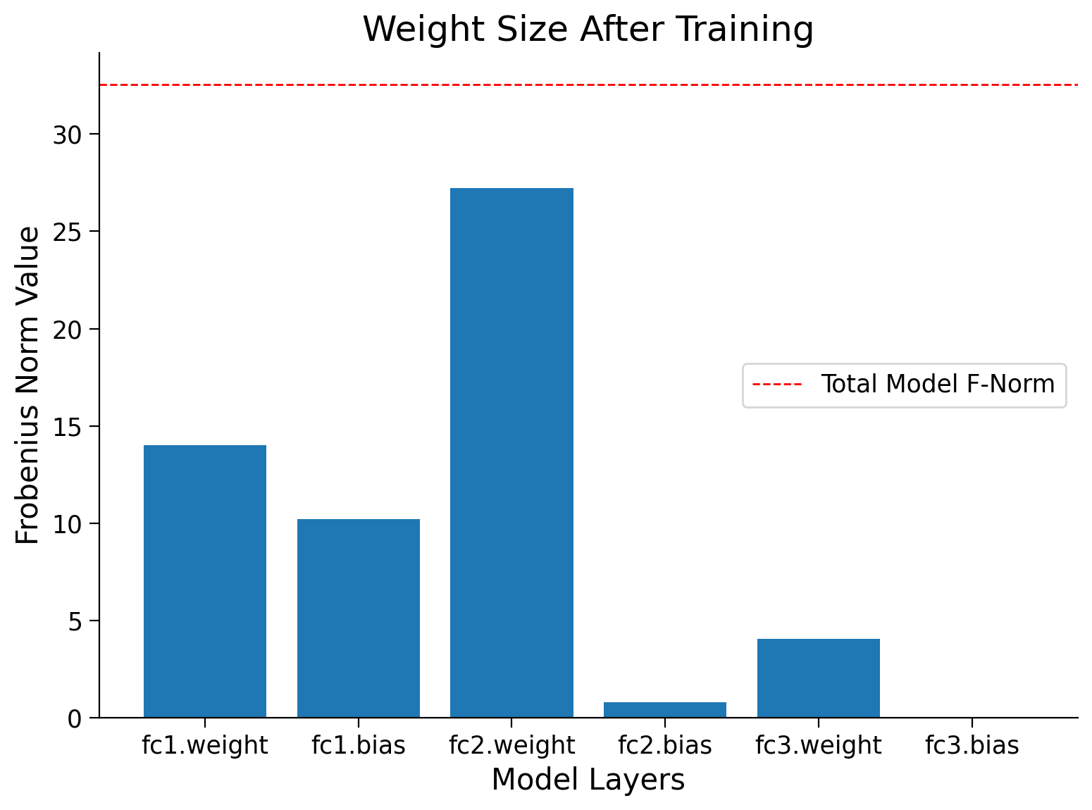
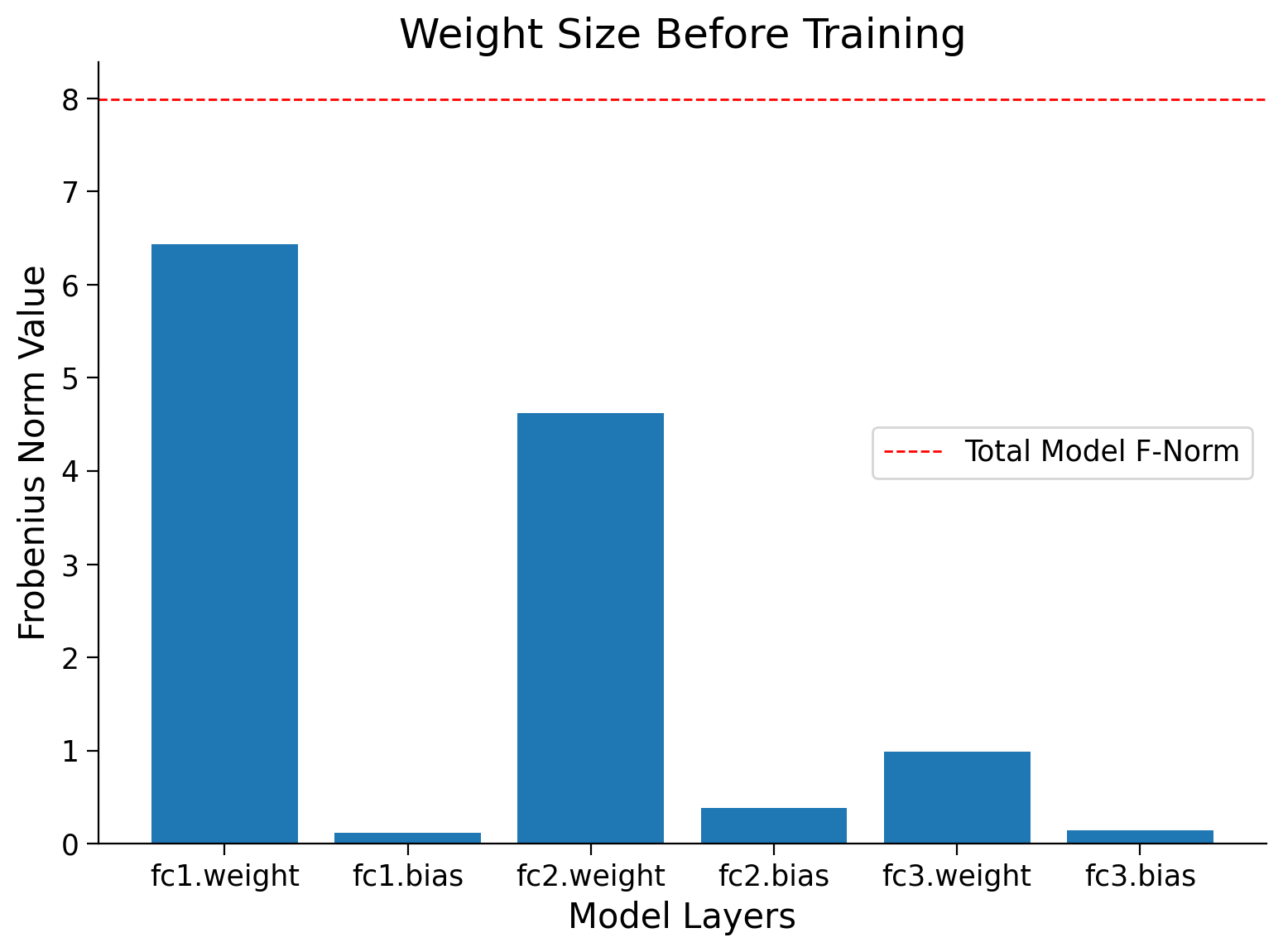
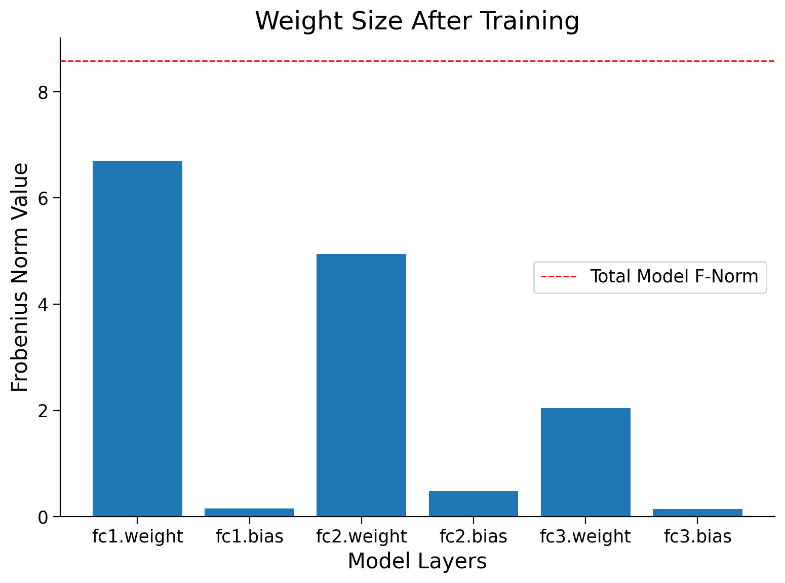
Finally, you can compare the Frobenius norm per layer in the model, before and after training.

Frobenius norm per layer before and after training

../../../_images/f7677587eea0099d87ca72136e5798438cc531f37a309517501b606513a5fb2d.png

../../../_images/096424eaa56ce6bb1650b00527c1964ed06db0349fcf1d81cfe3926ced2d0ebd.png

Section 2.2: Overfitting on Test Dataset#

In principle, we should not touch our test set until choosing all our hyperparameters. Were we to use the test data in the model selection process, there is a risk that we might overfit the test data, and then we will be in serious trouble. If we overfit our training data, there is always an evaluation using the test data to keep us honest. But if we overfit the test data, how would we ever know?

Note that there is another kind of overfitting: you do “honest” fitting on one set of images or posts or medical records, but it may not generalize to other images, posts, or medical records.

Validation Dataset#

A common practice to address this problem is to split our data in three ways, using a validation dataset (or validation set) to tune the hyperparameters. Ideally, we would only touch the test data once, to assess the very best model or to compare a small number of models to each other, real-world test data is seldom discarded after just one use.

Section 3: Memorization#

Time estimate: ~20 mins

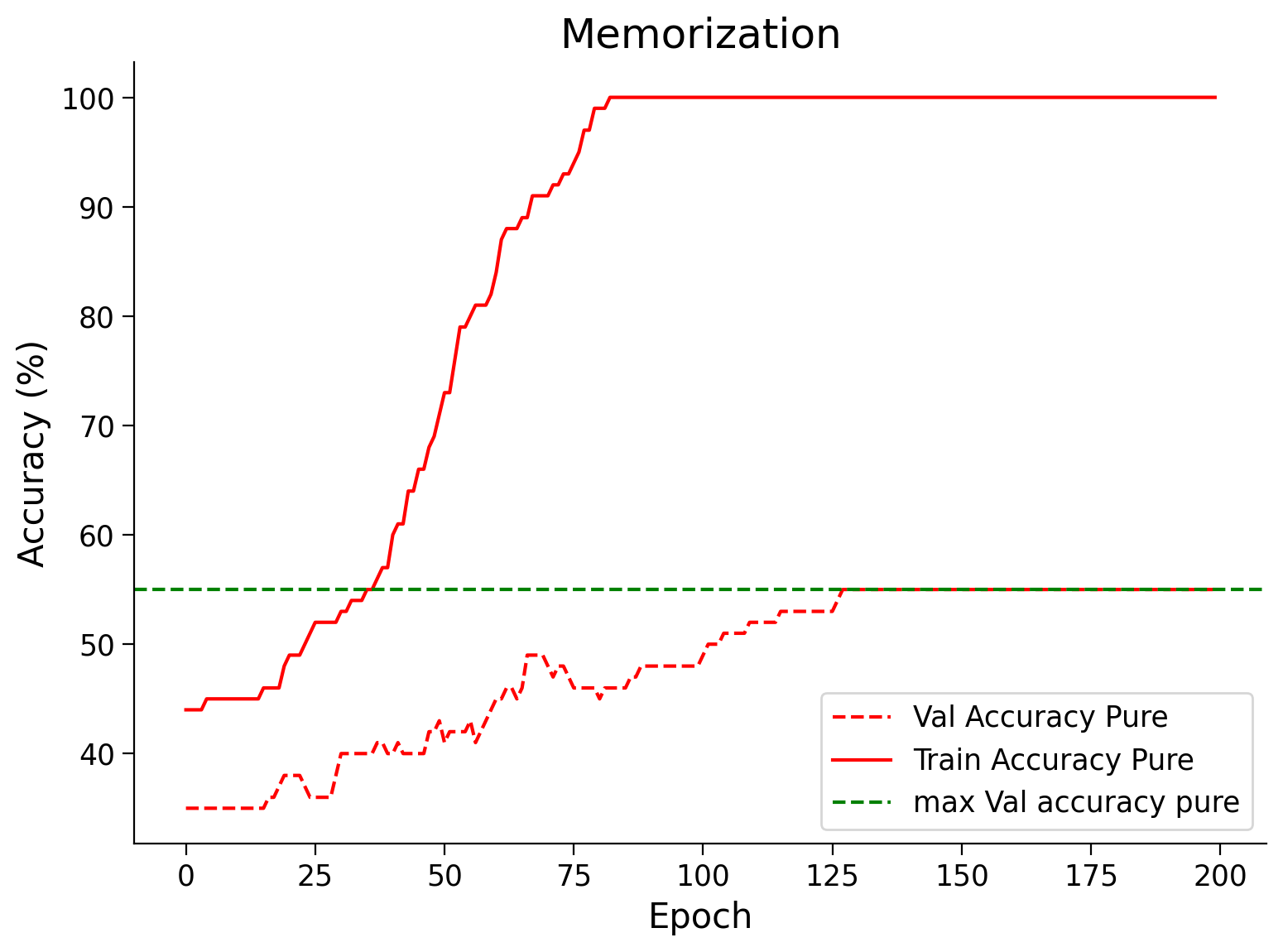
Given sufficiently large networks and enough training, Neural Networks can achieve almost 100% train accuracy by remembering each training example. However, this is bad because it will mean that the model will fail when presented with new data.

In this section, we train three MLPs; one each on:

Animal Faces Dataset
A Completely Noisy Dataset (Random shuffling of all labels)
A partially Noisy Dataset (Random shuffling of 15% labels)

Now, think for a couple of minutes as to what the train and test accuracies of each of these models might be, given that you train for sufficient time and use a powerful network.

First, let’s create the required dataloaders for all three datasets. Notice how we split the data. We train on a fraction of the dataset as it will be faster to train and will overfit more clearly.

# Dataloaders for the Dataset
batch_size = 128
classes = ('cat', 'dog', 'wild')

# Defining number of examples for train, val test
len_train, len_val, len_test = 100, 100, 14430

train_transform = transforms.Compose([
     transforms.ToTensor(),
     transforms.Normalize((0.5, 0.5, 0.5), (0.5, 0.5, 0.5))
     ])
data_path = pathlib.Path('.')/'afhq'  # Using pathlib to be compatible with all OS's
img_dataset = ImageFolder(data_path/'train', transform=train_transform)

# Dataloaders for the Original Dataset

# For reproducibility
g_seed = torch.Generator()
g_seed.manual_seed(SEED)

img_train_data, img_val_data,_ = torch.utils.data.random_split(img_dataset,
                                                               [len_train,
                                                                len_val,
                                                                len_test])

# Creating train_loader and Val_loader
train_loader = torch.utils.data.DataLoader(img_train_data,
                                           batch_size=batch_size,
                                           num_workers=2,
                                           worker_init_fn=seed_worker,
                                           generator=g_seed)

val_loader = torch.utils.data.DataLoader(img_val_data,
                                         batch_size=1000,
                                         num_workers=2,
                                         worker_init_fn=seed_worker,
                                         generator=g_seed)

# Dataloaders for the Random Dataset

# For reproducibility
g_seed = torch.Generator()
g_seed.manual_seed(SEED + 1)

# Splitting randomized data into training and validation data
data_path = pathlib.Path('.')/'afhq_random_32x32/afhq_random' # Using pathlib to be compatible with all OS's
img_dataset = ImageFolder(data_path/'train', transform=train_transform)
random_img_train_data, random_img_val_data,_ = torch.utils.data.random_split(img_dataset, [len_train, len_val, len_test])

# Randomized train and validation dataloader
rand_train_loader = torch.utils.data.DataLoader(random_img_train_data,
                                                batch_size=batch_size,
                                                num_workers=2,
                                                worker_init_fn=seed_worker,
                                                generator=g_seed)

rand_val_loader = torch.utils.data.DataLoader(random_img_val_data,
                                              batch_size=1000,
                                              num_workers=2,
                                              worker_init_fn=seed_worker,
                                              generator=g_seed)

# Dataloaders for the Partially Random Dataset

# For reproducibility
g_seed = torch.Generator()
g_seed.manual_seed(SEED + 1)

# Splitting data between training and validation dataset for partially randomized data
data_path = pathlib.Path('.')/'afhq_10_32x32/afhq_10' # Using pathlib to be compatible with all OS's
img_dataset = ImageFolder(data_path/'train', transform=train_transform)
partially_random_train_data, partially_random_val_data,_ = torch.utils.data.random_split(img_dataset, [len_train, len_val, len_test])

# Training and Validation loader for partially randomized data
partial_rand_train_loader = torch.utils.data.DataLoader(partially_random_train_data,
                                                        batch_size=batch_size,
                                                        num_workers=2,
                                                        worker_init_fn=seed_worker,
                                                        generator=g_seed)

partial_rand_val_loader = torch.utils.data.DataLoader(partially_random_val_data,
                                                      batch_size=1000,
                                                      num_workers=2,
                                                      worker_init_fn=seed_worker,
                                                      generator=g_seed)

Now let’s define a model which has many parameters compared to the training dataset size, and train it on these datasets.

class BigAnimalNet(nn.Module):
  """
  Network Class - Animal Faces with following structure:
  nn.Linear(3*32*32, 124) + leaky_relu(self.fc1(x)) # First fully connected layer
  nn.Linear(124, 64) + leaky_relu(self.fc2(x)) # Second fully connected layer
  nn.Linear(64, 3) # Final fully connected layer
  """

  def __init__(self):
    """
    Initialize parameters for BigAnimalNet

    Args:
      None

    Returns:
      Nothing
    """
    super(BigAnimalNet, self).__init__()
    self.fc1 = nn.Linear(3*32*32, 124)
    self.fc2 = nn.Linear(124, 64)
    self.fc3 = nn.Linear(64, 3)

  def forward(self, x):
    """
    Forward pass of BigAnimalNet

    Args:
      x: torch.tensor
        Input features

    Returns:
      x: torch.tensor
        Output/Predictions
    """
    x = x.view(x.shape[0], -1)
    x = F.leaky_relu(self.fc1(x))
    x = F.leaky_relu(self.fc2(x))
    x = self.fc3(x)
    output = F.log_softmax(x, dim=1)
    return output

Before training our BigAnimalNet(), calculate the Frobenius norm again.

set_seed(seed=SEED)
normi, wsi, label = calculate_frobenius_norm(BigAnimalNet())

Random seed 2021 has been set.

Now, train our BigAnimalNet() model

# Here we have 100 true train data.

# Set the arguments
args = {
    'epochs': 200,
    'lr': 5e-3,
    'momentum': 0.9,
    'device': DEVICE
}


# Initialize the network
set_seed(seed=SEED)
model = BigAnimalNet()

start_time = time.time()

# Train the network
val_acc_pure, train_acc_pure, _, model = main(args=args,
                                              model=model,
                                              train_loader=train_loader,
                                              val_loader=val_loader)
end_time = time.time()

print(f"Time to memorize the dataset: {end_time - start_time}")

# Train and Test accuracy plot
plt.figure(figsize=(8, 6))
plt.plot(val_acc_pure, label='Val Accuracy Pure', c='red', ls='dashed')
plt.plot(train_acc_pure, label='Train Accuracy Pure', c='red', ls='solid')
plt.axhline(y=max(val_acc_pure), c='green', ls='dashed',
            label='max Val accuracy pure')
plt.title('Memorization')
plt.ylabel('Accuracy (%)')
plt.xlabel('Epoch')
plt.legend()
plt.show()

Random seed 2021 has been set.

Time to memorize the dataset: 225.04949498176575

../../../_images/8ae7cd982c48a5de102c8d6905769be84e5acc537ae8b89cd6292cd2f0993030.png

Frobenius norm for AnimalNet before and after training#

../../../_images/da42e2626a961a450ddd110e5ba09e05e306fde26455d97b2eb04873f11bbfc0.png

../../../_images/7115401207a7c015679b0137158af5a34f99ab1c583958840de04e8653a18543.png

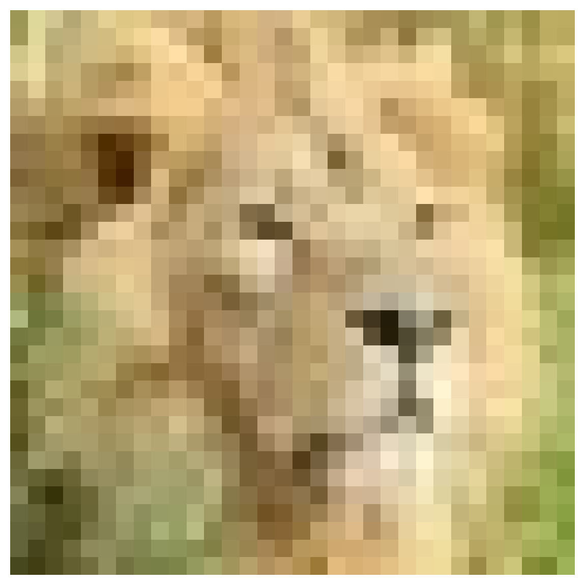
Data Visualizer#

Before we train the model on data with random labels, let’s visualize and verify for ourselves that the data is random. Here, we have:

classes = ("cat", "dog", "wild")

We use the .permute() method. plt.imshow() expects the input to be in NumPy format and in the format \((P_x, P_y, 3)\), where \(P_x\) and \(P_y\) are the number of pixels along \(x\) and \(y\) axis, respectively.

def visualize_data(dataloader):
  """
  Helper function to visualize data

  Args:
    dataloader: torch.tensor
      Dataloader to visualize

  Returns:
    Nothing
  """

  for idx, (data, label) in enumerate(dataloader):
    plt.figure(idx)

    # Choose the datapoint you would like to visualize
    index = 22

    # Choose that datapoint using index and permute the dimensions
    # and bring the pixel values between [0, 1]
    data = data[index].permute(1, 2, 0) * \
           torch.tensor([0.5, 0.5, 0.5]) + \
           torch.tensor([0.5, 0.5, 0.5])

    # Convert the torch tensor into numpy
    data = data.numpy()

    plt.imshow(data)
    plt.axis(False)
    image_class = classes[label[index].item()]
    print(f'The image belongs to : {image_class}')

  plt.show()


# Call the function
visualize_data(rand_train_loader)

The image belongs to : cat

../../../_images/2e0155f095b8d0008f42c3e8e6d2607c01f87f0e446fed56b38405866f541fb3.png

Now let’s train the network on the shuffled data and see if it memorizes.

# Here we have 100 completely shuffled train data.

# Set the arguments
args = {
    'epochs': 200,
    'lr': 5e-3,
    'momentum': 0.9,
    'device': DEVICE
}

# Initialize the model
set_seed(seed=SEED)
model = BigAnimalNet()

# Train the model
val_acc_random, train_acc_random, _, model = main(args,
                                                  model,
                                                  rand_train_loader,
                                                  val_loader)

# Train and Test accuracy plot
plt.figure(figsize=(8, 6))
plt.plot(val_acc_pure,label='Val - Pure',c='red',ls = 'dashed')
plt.plot(train_acc_pure,label='Train - Pure',c='red',ls = 'solid')
plt.plot(val_acc_random,label='Val - Random',c='blue',ls = 'dashed')
plt.plot(train_acc_random,label='Train - Random',c='blue',ls = 'solid')

plt.title('Memorization')
plt.ylabel('Accuracy (%)')
plt.xlabel('Epoch')
plt.legend()
plt.show()

Random seed 2021 has been set.

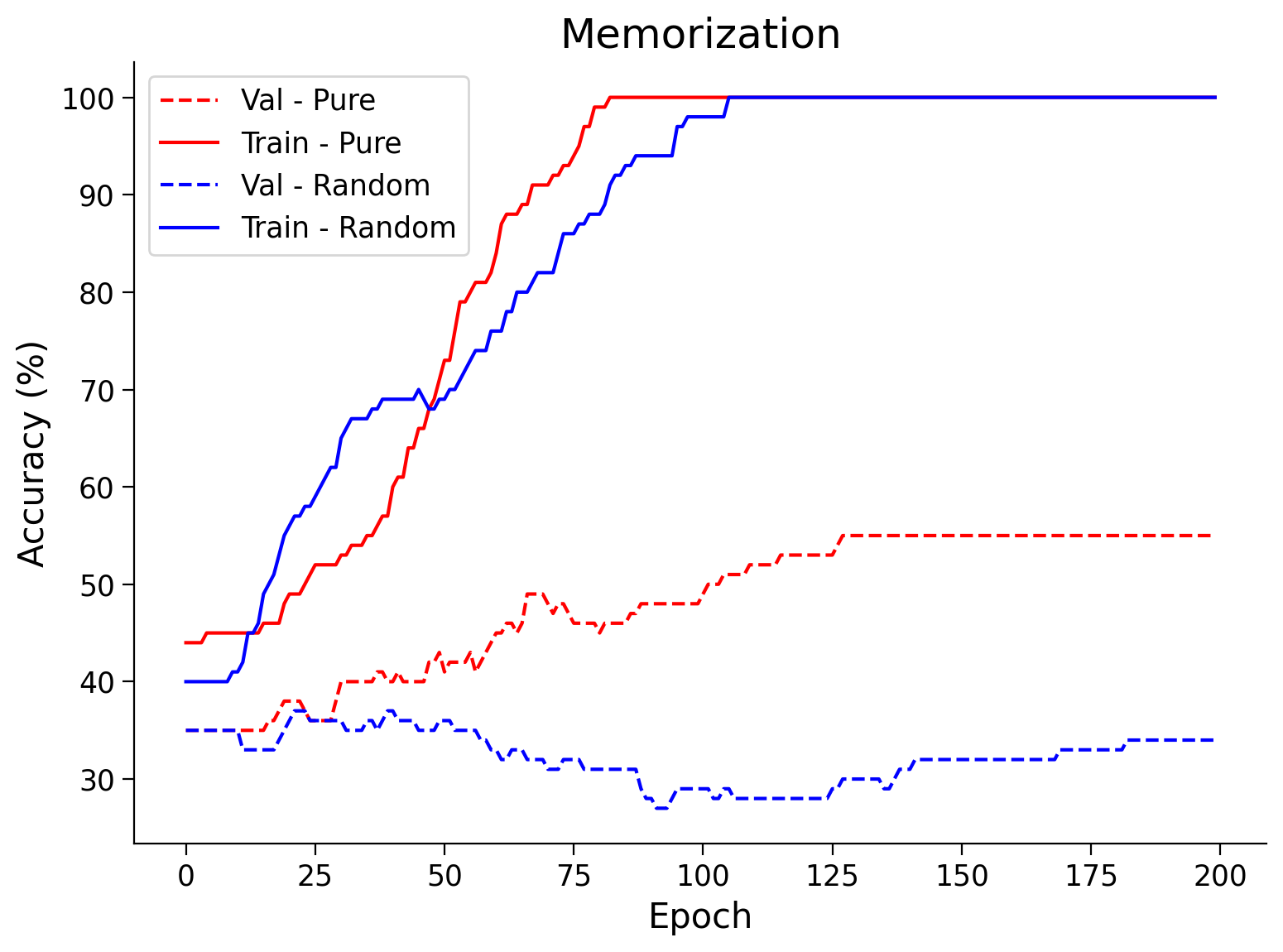
../../../_images/f39b59eb6c7c677dfbd0cccfa034f14897e0e44ce39cf11a9b5b0662b7e14383.png

Isn’t it surprising to see that the ANN was able to achieve 100% training accuracy on randomly shuffled labels? This is one of the reasons why training accuracy is not a good indicator of model performance.

Section 4: Early Stopping#

Time estimate: ~20 mins

Video 4: Early Stopping#

Submit your feedback#

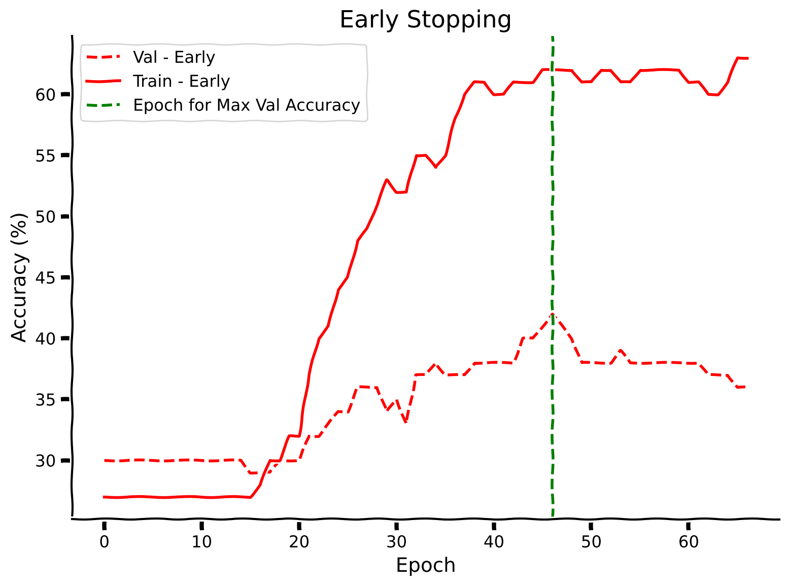
Now that we have established that the validation accuracy reaches the peak well before the model overfits, we want to stop the training somehow early. You should have also observed from the above plots that the train/test loss on real data is not very smooth, and hence you might guess that the choice of the epoch can play a crucial role in the validation/test accuracy.

Early stopping stops training when the validation accuracies stop increasing.

Coding Exercise 4: Early Stopping#

Reimplement the main function to include early stopping as described above. Then run the code below to validate your implementation.

def early_stopping_main(args, model, train_loader, val_loader):
  """
  Function to simulate early stopping

  Args:
    args: dictionary
      Dictionary with epochs: 200, lr: 5e-3, momentum: 0.9, device: DEVICE
    model: nn.module
      Neural network instance
    train_loader: torch.loader
      Train dataset
    val_loader: torch.loader
      Validation set

  Returns:
    val_acc_list: list
      Val accuracy log until early stop point
    train_acc_list: list
      Training accuracy log until early stop point
    best_model: nn.module
      Model performing best with early stopping
    best_epoch: int
      Epoch at which early stopping occurs
  """

  ####################################################################
  # Fill in all missing code below (...),
  # then remove or comment the line below to test your function
  raise NotImplementedError("Complete the early_stopping_main function")
  ####################################################################
  device = args['device']
  model = model.to(device)
  optimizer = optim.SGD(model.parameters(),
                        lr=args['lr'],
                        momentum=args['momentum'])

  best_acc = 0.0
  best_epoch = 0

  # Number of successive epochs that you want to wait before stopping training process
  patience = 20

  # Keeps track of number of epochs during which the val_acc was less than best_acc
  wait = 0

  val_acc_list, train_acc_list = [], []
  for epoch in tqdm(range(args['epochs'])):

    # Train the model
    trained_model = ...

    # Calculate training accuracy
    train_acc = ...

    # Calculate validation accuracy
    val_acc = ...

    if (val_acc > best_acc):
      best_acc = val_acc
      best_epoch = epoch
      best_model = copy.deepcopy(trained_model)
      wait = 0
    else:
      wait += 1

    if (wait > patience):
      print(f'Early stopped on epoch: {epoch}')
      break

    train_acc_list.append(train_acc)
    val_acc_list.append(val_acc)

  return val_acc_list, train_acc_list, best_model, best_epoch



# Set the arguments
args = {
    'epochs': 200,
    'lr': 5e-4,
    'momentum': 0.99,
    'device': DEVICE
}

# Initialize the model
set_seed(seed=SEED)
model = AnimalNet()

## Uncomment to test
# val_acc_earlystop, train_acc_earlystop, best_model, best_epoch = early_stopping_main(args, model, train_loader, val_loader)
# print(f'Maximum Validation Accuracy is reached at epoch: {best_epoch:2d}')
# early_stop_plot(train_acc_earlystop, val_acc_earlystop, best_epoch)

Random seed 2021 has been set.

Click for solution

Submit your feedback#

Think! 4: Early Stopping#

Discuss among your pod why or why not:

Do you think early stopping can be harmful to training your network?

Click for solution

Submit your feedback#

Summary#

In this tutorial, you have been introduced to the regularization technique, described as shrinkage. We have learned about overfitting, one of the worst caveats in deep learning, and finally, we have learned a method of reducing overfitting in our models called early-stopping.

If you have time left, you can learn how a model behaves when is trained with randomized labels.

Bonus: Train with randomized labels#

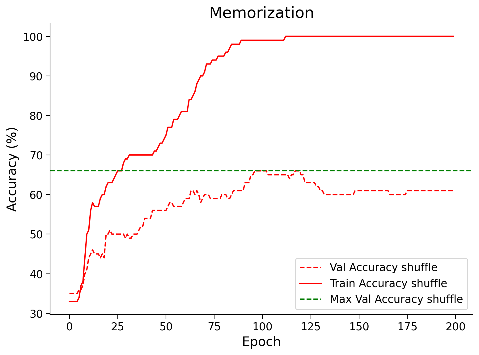
In this part, let’s train on a partially shuffled dataset where 15% of the labels are noisy.

# Here we have 15% partially shuffled train data.

# Set the arguments
args = {
    'epochs': 200,
    'lr': 5e-3,
    'momentum': 0.9,
    'device': DEVICE
}

# Intialize the model
set_seed(seed=SEED)
model = BigAnimalNet()

# Train the model
val_acc_shuffle, train_acc_shuffle, _, _, = main(args,
                                                 model,
                                                 partial_rand_train_loader,
                                                 val_loader)

# Train and test acc plot
plt.figure(figsize=(8, 6))
plt.plot(val_acc_shuffle, label='Val Accuracy shuffle', c='red', ls='dashed')
plt.plot(train_acc_shuffle, label='Train Accuracy shuffle', c='red', ls='solid')
plt.axhline(y=max(val_acc_shuffle), c='green', ls='dashed',
            label='Max Val Accuracy shuffle')
plt.title('Memorization')
plt.ylabel('Accuracy (%)')
plt.xlabel('Epoch')
plt.legend()
plt.show()

Random seed 2021 has been set.

../../../_images/ba1198882221690cb498e83f0ecebef51d6b091fcff67ca9438698ea18db5d67.png

Plotting them all together (Run Me!)#

../../../_images/48b2f3dcdc7f8ce5bfffc4c5841322d8b0dc4f8448f79906826ce8a8013cc772.png

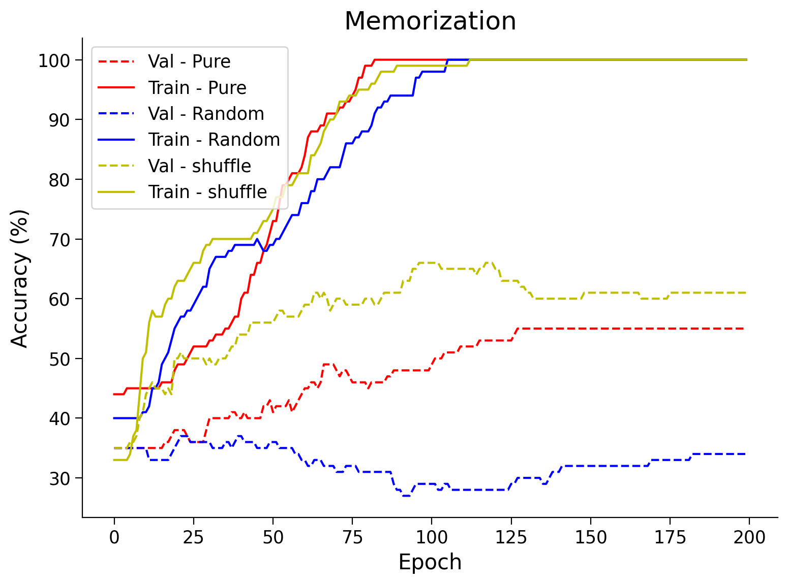
Think! Bonus: Does it Generalize?#

Given that the Neural Network fit/memorize the training data perfectly:

Do you think it generalizes well?
What makes you think it does or doesn’t?

Click for solution

Submit your feedback#

Also, it is interesting to note that sometimes the model trained on slightly shuffled data does slightly better than the one trained on pure data. Shuffling some of the data is a form of regularization, i.e., one of many ways of adding noise to the training data.

Tutorial 1: Regularization techniques part 1

Contents

Tutorial 1: Regularization techniques part 1#

Tutorial Objectives#

Setup#

Install dependencies#

Install and import feedback gadget#

Figure Settings#

Loading Animal Faces data#

Loading Animal Faces Randomized data#

Plotting functions#

Set random seed#

Set device (GPU or CPU). Execute set_device()#

Section 0: Defining useful functions#

Section 1: Regularization is Shrinkage#

Video 1: Introduction to Regularization#

Submit your feedback#

Video 2: Regularization as Shrinkage#

Submit your feedback#

Coding Exercise 1: Frobenius Norm#

Submit your feedback#

Section 2: Overfitting#

Video 3: Overparameterization and Overfitting#

Submit your feedback#

Section 2.1: Visualizing Overfitting#

Animation (Run Me!)#

Plot the train and test losses#

Think! 2.1: Interpreting losses#

Submit your feedback#

Section 2.2: Overfitting on Test Dataset#

Validation Dataset#

Section 3: Memorization#

Frobenius norm for AnimalNet before and after training#

Data Visualizer#

Section 4: Early Stopping#

Video 4: Early Stopping#

Submit your feedback#

Coding Exercise 4: Early Stopping#

Submit your feedback#

Think! 4: Early Stopping#

Submit your feedback#

Summary#

Bonus: Train with randomized labels#

Plotting them all together (Run Me!)#

Think! Bonus: Does it Generalize?#

Submit your feedback#

Set device (GPU or CPU). Execute `set_device()`#