Tutorial 1: Introduction to processing time series

Tutorial 1: Introduction to processing time series#

Week 3, Day 1: Time Series And Natural Language Processing

By Neuromatch Academy

Content creators: Lyle Ungar, Kelson Shilling-Scrivo, Alish Dipani

Content reviewers: Kelson Shilling-Scrivo

Content editors: Gagana B, Spiros Chavlis, Kelson Shilling-Scrivo

Production editors: Gagana B, Spiros Chavlis

Based on Content from: Anushree Hede, Pooja Consul, Ann-Katrin Reuel

Tutorial objectives#

Before we explore how Recurrent Neural Networks (RNNs) excel at modeling sequences, we will explore other ways to model sequences, encode the text, and make meaningful measurements using such encodings and embeddings.

Setup#

Install dependencies#

There may be errors and/or warnings reported during the installation. However, they are to be ignored.

Install and import feedback gadget#

Install fastText#

If you want to see the original code, go to GitHub repo.

Downloading Started...

Downloading Completed.
Extracting all the files now...
Done!

# Imports
import time
import nltk
import fasttext
import numpy as np
import matplotlib.pyplot as plt
from collections import Counter

from nltk.corpus import brown
from nltk.tokenize import word_tokenize
from gensim.models import Word2Vec

import torch.nn as nn
from torch.nn import functional as F
from torch.utils.data import DataLoader
from torch.nn.utils.rnn import pad_sequence

from torchtext import datasets
from torchtext.vocab import FastText
from torchtext.vocab import vocab as Vocab
from torchtext.datasets import IMDB, AG_NEWS
from torchtext.data.utils import get_tokenizer
from torch.utils.data.dataset import random_split
from torchtext.vocab import build_vocab_from_iterator
from torchtext.data.functional import to_map_style_dataset

---------------------------------------------------------------------------
ImportError                               Traceback (most recent call last)
Cell In[5], line 11
      9 from nltk.corpus import brown
     10 from nltk.tokenize import word_tokenize
---> 11 from gensim.models import Word2Vec
     13 import torch.nn as nn
     14 from torch.nn import functional as F

File /opt/hostedtoolcache/Python/3.9.19/x64/lib/python3.9/site-packages/gensim/__init__.py:11
      7 __version__ = '4.3.2'
      9 import logging
---> 11 from gensim import parsing, corpora, matutils, interfaces, models, similarities, utils  # noqa:F401
     14 logger = logging.getLogger('gensim')
     15 if not logger.handlers:  # To ensure reload() doesn't add another one

File /opt/hostedtoolcache/Python/3.9.19/x64/lib/python3.9/site-packages/gensim/corpora/__init__.py:6
      1 """
      2 This package contains implementations of various streaming corpus I/O format.
      3 """
      5 # bring corpus classes directly into package namespace, to save some typing
----> 6 from .indexedcorpus import IndexedCorpus  # noqa:F401 must appear before the other classes
      8 from .mmcorpus import MmCorpus  # noqa:F401
      9 from .bleicorpus import BleiCorpus  # noqa:F401

File /opt/hostedtoolcache/Python/3.9.19/x64/lib/python3.9/site-packages/gensim/corpora/indexedcorpus.py:14
     10 import logging
     12 import numpy
---> 14 from gensim import interfaces, utils
     16 logger = logging.getLogger(__name__)
     19 class IndexedCorpus(interfaces.CorpusABC):

File /opt/hostedtoolcache/Python/3.9.19/x64/lib/python3.9/site-packages/gensim/interfaces.py:19
      7 """Basic interfaces used across the whole Gensim package.
      8 
      9 These interfaces are used for building corpora, model transformation and similarity queries.
   (...)
     14 
     15 """
     17 import logging
---> 19 from gensim import utils, matutils
     22 logger = logging.getLogger(__name__)
     25 class CorpusABC(utils.SaveLoad):

File /opt/hostedtoolcache/Python/3.9.19/x64/lib/python3.9/site-packages/gensim/matutils.py:20
     18 import scipy.sparse
     19 from scipy.stats import entropy
---> 20 from scipy.linalg import get_blas_funcs, triu
     21 from scipy.linalg.lapack import get_lapack_funcs
     22 from scipy.special import psi  # gamma function utils

ImportError: cannot import name 'triu' from 'scipy.linalg' (/opt/hostedtoolcache/Python/3.9.19/x64/lib/python3.9/site-packages/scipy/linalg/__init__.py)

Figure Settings#

Load Dataset from `nltk`#

True

Helper functions#

Set random seed#

Executing set_seed(seed=seed) you are setting the seed

Set device (GPU or CPU). Execute `set_device()`#

DEVICE = set_device()
SEED = 2021
set_seed(seed=SEED)

WARNING: For this notebook to perform best, if possible, in the menu under `Runtime` -> `Change runtime type.`  select `GPU` 
Random seed 2021 has been set.

Section 1: Intro: What time series are there?#

Time estimate: 20 mins

Video 1: Time Series and NLP#

Submit your feedback#

Video 2: What is NLP?#

Submit your feedback#

Section 2: Embeddings#

Time estimate: 50 mins

Video 3: NLP Tokenization#

Submit your feedback#

Section 2.1: Introduction#

Word2vec is a group of related models that produce word embeddings. These models are shallow, two-layer neural networks trained to reconstruct linguistic contexts of words. Word2vec takes a large corpus of text as input and produces a vector space, with each unique word in the corpus being assigned a corresponding vector in the space.

Creating Word Embeddings#

We will create embeddings for a subset of categories in Brown corpus. To achieve this task we will use gensim library to create word2vec embeddings. Gensim’s word2vec expects a sequence of sentences as its input. Each sentence is a list of words.

Calling Word2Vec(sentences, iter=1) will run two passes over the sentences iterator (generally, iter+1 passes). The first pass collects words and their frequencies to build an internal dictionary tree structure. The second and subsequent passes train the neural model. Word2vec accepts several parameters that affect both training speed and quality.

One of them is for pruning the internal dictionary. Words that appear only once or twice in a billion-word corpus are probably uninteresting typos and garbage. In addition, there are not enough data to make any meaningful training on those words, so it’s best to ignore them:

model = Word2Vec(sentences, min_count=10)  # default value is 5

A reasonable value for min_count is bewteen 0-100, depending on the size of your dataset.

Another parameter is the size of the NN layers, which correspond to the “degrees” of freedom the training algorithm has:

model = Word2Vec(sentences, size=200)  # default value is 100

Bigger size values require more training data but can lead to better (more accurate) models. Reasonable values are in the tens to hundreds.

The last of the major parameters (full list here) is for training parallelization, to speed up training:

model = Word2Vec(sentences, workers=4)  # default = 1 worker = no parallelization

# Categories used for the Brown corpus
category = ['editorial', 'fiction', 'government', 'mystery', 'news', 'religion',
            'reviews', 'romance', 'science_fiction']

Word2Vec model

The cell will take 30-45 seconds to run.

# Create a word2vec model based on categories from Brown corpus
w2vmodel = create_word2vec_model(category)

You can get the embedding vector for a word in the dictionary.

# get word list from Brown corpus
brown_wordlist = list(brown.words(categories=category))
# generate a random word
random_word = random.sample(brown_wordlist, 1)[0]
# get embedding of the random word
random_word_embedding = get_embedding(random_word, w2vmodel)
print(f'Embedding of "{random_word}" is {random_word_embedding}')

Visualizing Word Embeddings#

We can now obtain the word embeddings for any word in the dictionary using word2vec. Let’s visualize these embeddings to get an intuition of what these embeddings mean. The word embeddings obtained from the word2vec model are in high dimensional space, and we will use tSNE to pick the two features that capture the most variance in the embeddings to represent them in a 2D space.

For each word in keys, we pick the top 10 similar words (using cosine similarity) and plot them.

Before you run the code, spend some time to think:

What should be the arrangement of similar words?
What should be the arrangement of the critical clusters with respect to each other?

keys = ['voters', 'magic', 'love', 'God', 'evidence', 'administration', 'governments']

Show code cell source Hide code cell source

# @markdown ### Cluster embeddings related functions

# @markdown **Note:** We import [sklearn.manifold.TSNE](https://scikit-learn.org/stable/modules/generated/sklearn.manifold.TSNE.html)
from sklearn.manifold import TSNE
import matplotlib.cm as cm

def get_cluster_embeddings(keys):
  embedding_clusters = []
  word_clusters = []

  # find closest words and add them to cluster
  for word in keys:
    embeddings = []
    words = []
    if not word in w2vmodel.wv:
      print(f'The word {word} is not in the dictionary')
      continue

    for similar_word, _ in w2vmodel.wv.most_similar(word, topn=10):
      words.append(similar_word)
      embeddings.append(w2vmodel.wv[similar_word])
    embeddings.append(get_embedding(word, w2vmodel))
    words.append(word)
    embedding_clusters.append(embeddings)
    word_clusters.append(words)

  # get embeddings for the words in clusers
  embedding_clusters = np.array(embedding_clusters)
  n, m, k = embedding_clusters.shape
  tsne_model_en_2d = TSNE(perplexity=10, n_components=2, init='pca', n_iter=3500, random_state=32)
  embeddings_en_2d = np.array(tsne_model_en_2d.fit_transform(embedding_clusters.reshape(n * m, k))).reshape(n, m, 2)
  return embeddings_en_2d, word_clusters


def tsne_plot_similar_words(title, labels, embedding_clusters,
                            word_clusters, opacity, filename=None):
  plt.figure(figsize=(16, 9))
  colors = cm.rainbow(np.linspace(0, 1, len(labels)))
  for label, embeddings, words, color in zip(labels, embedding_clusters, word_clusters, colors):
    x = embeddings[:, 0]
    y = embeddings[:, 1]
    plt.scatter(x, y, color=color, alpha=opacity, label=label)
    # Plot the cluster centroids
    plt.plot(np.mean(x), np.mean(y), 'x', color=color, markersize=16)
    for i, word in enumerate(words):
      size = 10 if i < 10 else 14
      plt.annotate(word, alpha=0.5, xy=(x[i], y[i]), xytext=(5, 2),
                    textcoords='offset points',
                    ha='right', va='bottom', size=size)
  plt.legend()
  plt.title(title)
  plt.grid(True)
  if filename:
    plt.savefig(filename, format='png', dpi=150, bbox_inches='tight')
  plt.show()

# Get closest words to the keys and get clusters of these words
embeddings_en_2d, word_clusters = get_cluster_embeddings(keys)
# tSNE plot of similar words to keys
tsne_plot_similar_words(title='Similar words from Brown Corpus',
                        labels=keys,
                        embedding_clusters=embeddings_en_2d,
                        word_clusters=word_clusters,
                        opacity=0.7,
                        filename='similar_words.png')

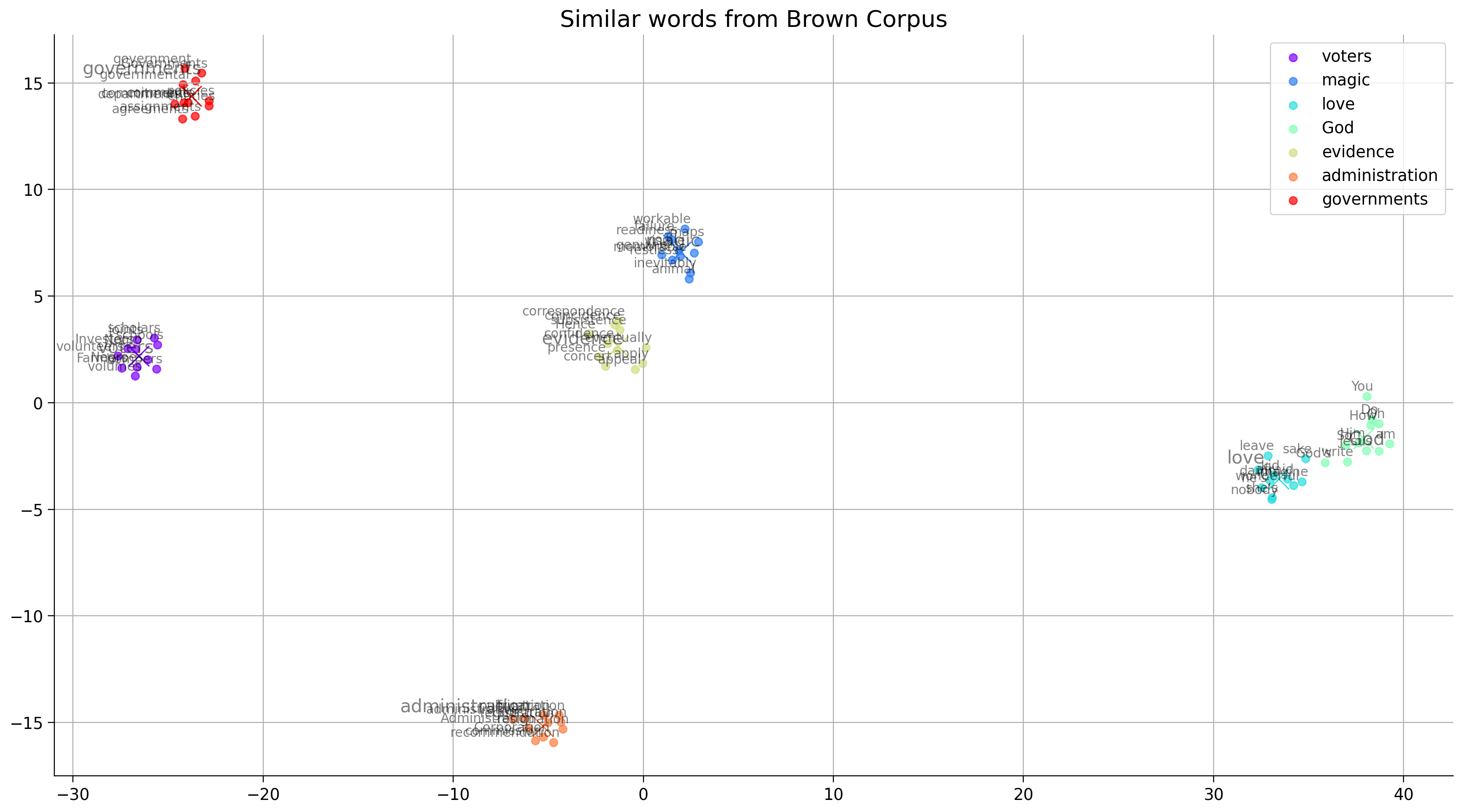
Think! 2.1: Similarity#

What does having higher similarity between two word embeddings mean?
Why are cluster centroids (represented with X in the plot) close to some keys (represented with larger fonts) but farther from others?

Click for solution

Submit your feedback#

Section 2.2: Embedding exploration#

Video 4: Embeddings rule!#

Submit your feedback#

Video 5: Distributional Similarity and Vector Embeddings#

Submit your feedback#

Words or subword units such as morphemes are the basic units we use to express meaning in language. The technique of mapping words to vectors of real numbers is known as word embedding.

In this section, we will use pretrained fastText embeddings, a context-oblivious embedding similar to word2vec.

Embedding Manipulation#

Let’s use the FastText library to manipulate the embeddings. First, find the embedding for the word “King”

Downloading Started...

Downloading Completed.
Extracting all the files now...

Done!

# Load 100 dimension FastText Vectors using FastText library
ft_en_vectors = fasttext.load_model('cc.en.100.bin')
print(f"Length of the embedding is: {len(ft_en_vectors.get_word_vector('king'))}")
print(f"\nEmbedding for the word King is:\n {ft_en_vectors.get_word_vector('king')}")

Length of the embedding is: 100

Embedding for the word King is:
 [-0.04045481 -0.10617249 -0.27222311  0.06879666  0.16408321  0.00276707
  0.27080125 -0.05805573 -0.31865698  0.03748008 -0.00254088  0.13805169
 -0.00182498 -0.08973497  0.00319015 -0.19619396 -0.09858181 -0.10103802
 -0.08279888  0.0082208   0.13119364 -0.15956607  0.17203182  0.0315701
 -0.25064597  0.06182072  0.03929246  0.05157393  0.03543638  0.13660161
  0.05473648  0.06072914 -0.04709269  0.17394426 -0.02101276 -0.11402624
 -0.24489872 -0.08576579 -0.00322696 -0.04509873 -0.00614253 -0.05772085
 -0.073414   -0.06718913 -0.06057961  0.10963406  0.1245006  -0.04819863
  0.11408057  0.11081408  0.06752145 -0.01689911 -0.01186301 -0.11716368
 -0.01287614  0.10639337 -0.04243141  0.01057278 -0.0230855  -0.04930984
  0.04717607  0.03696446  0.0015999  -0.02193867 -0.01331578  0.11102925
  0.1686794   0.05814958 -0.00296521 -0.04252011 -0.00352389  0.06267346
 -0.07747819 -0.08959802 -0.02445797 -0.08913022  0.13422231  0.1258949
 -0.01296814  0.0531218  -0.00541025 -0.16908626  0.06323182 -0.11510128
 -0.08352032 -0.07224389  0.01023453  0.08263734 -0.03859017 -0.00798539
 -0.01498295  0.05448429  0.02708506  0.00549948  0.14634523 -0.12550676
  0.04641578 -0.10164826  0.05370862  0.01217492]

Cosine similarity is used for similarities between words. Similarity is a scalar between 0 and 1. Higher scalar value corresponds to higher similarity.

Now find the 10 most similar words to “king”.

ft_en_vectors.get_nearest_neighbors("king", 10)  # Most similar by key

[(0.8168574571609497, 'prince'),
 (0.796097457408905, 'emperor'),
 (0.7907207608222961, 'kings'),
 (0.7655220627784729, 'lord'),
 (0.7435404062271118, 'king-'),
 (0.7394551634788513, 'chieftain'),
 (0.7307553291320801, 'tyrant'),
 (0.7226710319519043, 'conqueror'),
 (0.719561755657196, 'kingly'),
 (0.718187689781189, 'queen')]

Word Similarity#

More on similarity between words. Let’s check how similar different pairs of word are.

def cosine_similarity(vec_a, vec_b):
  """Compute cosine similarity between vec_a and vec_b"""
  return np.dot(vec_a, vec_b) / (np.linalg.norm(vec_a) * np.linalg.norm(vec_b))


def getSimilarity(word1, word2):
  v1 = ft_en_vectors.get_word_vector(word1)
  v2 = ft_en_vectors.get_word_vector(word2)
  return cosine_similarity(v1, v2)


print(f"Similarity between the words King and Queen: {getSimilarity('king', 'queen')}")
print(f"Similarity between the words King and Knight: {getSimilarity('king', 'knight')}")
print(f"Similarity between the words King and Rock: {getSimilarity('king', 'rock')}")
print(f"Similarity between the words King and Twenty: {getSimilarity('king', 'twenty')}")

print(f"\nSimilarity between the words Dog and Cat: {getSimilarity('dog', 'cat')}")
print(f"Similarity between the words Ascending and Descending: {getSimilarity('ascending', 'descending')}")
print(f"Similarity between the words Victory and Defeat: {getSimilarity('victory', 'defeat')}")
print(f"Similarity between the words Less and More: {getSimilarity('less', 'more')}")
print(f"Similarity between the words True and False: {getSimilarity('true', 'false')}")

Similarity between the words King and Queen: 0.7181877493858337
Similarity between the words King and Knight: 0.6881008744239807
Similarity between the words King and Rock: 0.2892838716506958
Similarity between the words King and Twenty: 0.19655467569828033

Similarity between the words Dog and Cat: 0.833964467048645
Similarity between the words Ascending and Descending: 0.8707448840141296
Similarity between the words Victory and Defeat: 0.7478055953979492
Similarity between the words Less and More: 0.8461978435516357
Similarity between the words True and False: 0.595384955406189

Interactive Demo 2.2.1: Check similarity between words#

Type two words and run the cell!

Similarity between King and Frog: 0.5649225115776062

Using embeddings, we can find the words that appear in similar contexts. But, what happens if the word has several different meanings?

Homonym Similarity#

Homonyms are words that have the same spelling or pronunciation but different meanings depending on the context. Let’s explore how these words are embedded and their similarity in different contexts.

#######################     Words with multiple meanings     ##########################
print(f"Similarity between the words Cricket and Insect: {getSimilarity('cricket', 'insect')}")
print(f"Similarity between the words Cricket and Sport: {getSimilarity('cricket', 'sport')}")

Similarity between the words Cricket and Insect: 0.4072215259075165
Similarity between the words Cricket and Sport: 0.5812374353408813

Submit your feedback#

Interactive Demo 2.2.2: Explore homonyms#

Similarity between minute and time: 0.7297980785369873
Similarity between minute and small: 0.340322345495224

Word Analogies#

Embeddings can be used to find word analogies. Let’s try it:

Man : Woman :: King : _____
Germany: Berlin :: France : _____
Leaf : Tree :: Petal : _____

## Use get_analogies() funnction.
# The words have to be in the order Positive, negative,  Positve

# Man : Woman  ::  King : _____
# Positive=(woman, king), Negative=(man)
print(ft_en_vectors.get_analogies("woman", "man", "king", 1))

# Germany: Berlin :: France : ______
# Positive=(berlin, frannce), Negative=(germany)
print(ft_en_vectors.get_analogies("berlin", "germany", "france", 1))

# Leaf : Tree  ::  Petal : _____
# Positive=(tree, petal), Negative=(leaf)
print(ft_en_vectors.get_analogies("tree", "leaf", "petal", 1))

[(0.8162637948989868, 'queen')]
[(0.8568049669265747, 'paris')]
[(0.7037209272384644, 'flower')]

But, does it always work?

Poverty : Wealth :: Sickness : _____
train : board :: horse : _____

# Poverty : Wealth  :: Sickness : _____
print(ft_en_vectors.get_analogies("wealth", "poverty", "sickness", 1))

# train : board :: horse : _____
print(ft_en_vectors.get_analogies("board", "train", "horse", 1))

[(0.615874171257019, 'affliction')]
[(0.5437814593315125, 'bull')]

Submit your feedback#

Section 2.3: Neural Net with word embeddings#

Video 6: Using Embeddings#

Submit your feedback#

Training context-oblivious word embeddings is relatively cheap, but most people still use pre-trained word embeddings. After we cover context-sensitive word embeddings, we’ll see how to “fine tune” embeddings (adjust them to the task at hand).

Let’s use the pretrained FastText embeddings to train a neural network on the IMDB dataset.

The data consists of reviews and sentiments attached to it, and it is a binary classification task.

Coding Exercise 1: Simple feed forward net#

Define a vanilla neural network with linear layers. Then average the word embeddings to get an embedding for the entire review. The neural net will have one hidden layer of size 128.

class NeuralNet(nn.Module):
  """ A vanilla neural network. """
  def __init__(self, output_size, hidden_size, vocab_size,
               embedding_length, word_embeddings):
    """
    Constructs a vanilla Neural Network Instance.

    Args:
      batch_size: Integer
        Specifies probability of dropout hyperparameter
      output_size: Integer
        Specifies the size of output vector
      hidden_size: Integer
        Specifies the size of hidden layer
      vocab_size: Integer
        Specifies the size of the vocabulary
        i.e. the number of tokens in the vocabulary
      embedding_length: Integer
        Specifies the size of the embedding vector
      word_embeddings
        Specifies the weights to create embeddings from
        voabulary.

    Returns:
      Nothing
    """
    super(NeuralNet, self).__init__()

    self.output_size = output_size
    self.hidden_size = hidden_size
    self.vocab_size = vocab_size
    self.embedding_length = embedding_length

    # self.word_embeddings = nn.EmbeddingBag(vocab_size, embedding_length, sparse=False)
    self.word_embeddings = nn.EmbeddingBag.from_pretrained(embedding_fasttext.vectors)
    self.word_embeddings.weight.requiresGrad = False
    self.fc1 = nn.Linear(embedding_length, hidden_size)
    self.fc2 = nn.Linear(hidden_size, output_size)
    self.init_weights()

  def init_weights(self):
      initrange = 0.5
      # self.word_embeddings.weight.data.uniform_(-initrange, initrange)
      self.fc1.weight.data.uniform_(-initrange, initrange)
      self.fc1.bias.data.zero_()
      self.fc2.weight.data.uniform_(-initrange, initrange)
      self.fc2.bias.data.zero_()

  def forward(self, inputs, offsets):
    """
    Compute the final labels by taking tokens as input.

    Args:
      inputs: Tensor
        Tensor of tokens in the text

    Returns:
      out: Tensor
        Final prediction Tensor
    """
    embedded = self.word_embeddings(inputs, offsets)  # convert text to embeddings
    #################################################
    # Implement a vanilla neural network
    raise NotImplementedError("Neural Net `forward`")
    #################################################
    # Pass the embeddings through the neural net
    # Use ReLU as the non-linearity
    x = ...
    x = ...
    x = ...
    output = F.log_softmax(x, dim=1)
    return output

Click for solution

Submit your feedback#

Show code cell source Hide code cell source

# @markdown ### Helper functions

# @markdown - `train(model, device, train_iter, valid_iter, epochs, learning_rate)`

# @markdown - `test(model,  device, test_iter)`

# @markdown - `load_dataset(emb_vectors, seed, batch_size=32)`

# @markdown - `plot_train_val(x, train, val, train_label, val_label, title)`


# Training
import time

def train(dataloader):
  model.train()
  total_acc, total_count = 0, 0
  running_loss = 0
  log_interval = 500
  start_time = time.time()

  for idx, (label, text, offsets) in enumerate(dataloader):
    optimizer.zero_grad()
    predicted_label = model(text, offsets)
    loss = criterion(predicted_label, label)
    loss.backward()
    torch.nn.utils.clip_grad_norm_(model.parameters(), 0.1)
    optimizer.step()
    total_acc += (predicted_label.argmax(1) == label).sum().item()
    total_count += label.size(0)
    if idx % log_interval == 0 and idx > 0:
      elapsed = time.time() - start_time
      print(f'| epoch {epoch:3d} | {idx:5d}/{len(dataloader):5d} batches '
            f'| accuracy {total_acc/total_count:8.3f}')

      start_time = time.time()

    running_loss += loss.item()
  return total_acc/total_count, loss


def evaluate(dataloader):
  model.eval()
  total_acc, total_count = 0, 0
  running_loss = 0

  with torch.no_grad():
    for idx, (label, text, offsets) in enumerate(dataloader):
      predicted_label = model(text, offsets)
      loss = criterion(predicted_label, label)
      total_acc += (predicted_label.argmax(1) == label).sum().item()
      total_count += label.size(0)
      running_loss += loss
  return total_acc/total_count, loss


def load_dataset(train_iter, device='cpu', seed=0, batch_size=32, valid_split=0.7):

  # Prepare data processing pipelines
  tokenizer = get_tokenizer('basic_english')

  def yield_tokens(data_iter):
      for _, text in data_iter:
          yield tokenizer(text)

  # Create a vocabulary block
  vocab = build_vocab_from_iterator(yield_tokens(train_iter), specials=["<unk>"])
  vocab.set_default_index(vocab["<unk>"])

  # Prepare the text processing pipeline with the tokenizer and vocabulary
  text_pipeline = lambda x: vocab(tokenizer(x))
  label_pipeline = lambda x: int(x) - 1

  def collate_batch(batch):
      label_list, text_list, offsets = [], [], [0]
      for (_label, _text) in batch:
          label_list.append(label_pipeline(_label))
          processed_text = torch.tensor(text_pipeline(_text), dtype=torch.int64)
          text_list.append(processed_text)
          offsets.append(processed_text.size(0))
      label_list = torch.tensor(label_list, dtype=torch.int64)
      offsets = torch.tensor(offsets[:-1]).cumsum(dim=0)
      text_list = torch.cat(text_list)
      return label_list.to(device), text_list.to(device), offsets.to(device)

  # Generate data batch and iterator and split the data
  train_iter, test_iter = AG_NEWS()
  train_dataset = to_map_style_dataset(train_iter)
  test_dataset = to_map_style_dataset(test_iter)
  num_train = int(len(train_dataset) * valid_split)
  num_valid = len(train_dataset) - num_train
  generator = torch.Generator().manual_seed(seed)
  split_train_, split_valid_ = random_split(train_dataset, [num_train, num_valid], generator=generator)

  train_dataloader = DataLoader(split_train_, batch_size=batch_size,
                                shuffle=True, collate_fn=collate_batch)
  valid_dataloader = DataLoader(split_valid_, batch_size=batch_size,
                                shuffle=True, collate_fn=collate_batch)
  test_dataloader = DataLoader(test_dataset, batch_size=batch_size,
                               shuffle=True, collate_fn=collate_batch)

  return vocab, train_dataloader, valid_dataloader, test_dataloader


# Plotting
def plot_train_val(x, train, val, train_label, val_label, title, ylabel):
  plt.plot(x, train, label=train_label)
  plt.plot(x, val, label=val_label)
  plt.legend()
  plt.xlabel('epoch')
  plt.ylabel(ylabel)
  plt.title(title)
  plt.show()


# Dataset
def tokenize(sentences):
  # Tokenize the sentence
  # from nltk.tokenize library use word_tokenize
  token = word_tokenize(sentences)
  return token

train_iter = AG_NEWS(split='train')
num_class = len(set([label for (label, text) in train_iter]))
vocab_size = len(VOCAB)
hidden_size = 128
embedding_length = 300
model = NeuralNet(num_class, hidden_size, vocab_size, embedding_length, embedding_fasttext).to(DEVICE)

# Hyperparameters
EPOCHS = 10  # epoch
LR = 5  # learning rate
BATCH_SIZE = 64  # batch size for training

criterion = torch.nn.CrossEntropyLoss()
optimizer = torch.optim.SGD(model.parameters(), lr=LR)
scheduler = torch.optim.lr_scheduler.StepLR(optimizer, 1.0, gamma=0.1)
total_accu = None

train_loss, val_loss = [], []
train_acc, val_acc = [], []

for epoch in range(1, EPOCHS + 1):
    epoch_start_time = time.time()
    accu_train, loss_train = train(train_data)
    accu_val, loss_val = evaluate(valid_data)
    train_loss.append(loss_train)
    val_loss.append(loss_val)
    train_acc.append(accu_train)
    val_acc.append(accu_val)

    if total_accu is not None and total_accu > accu_val:
      scheduler.step()
    else:
       total_accu = accu_val
    print('-' * 59)
    print('| end of epoch {:3d} | time: {:5.2f}s | '
          'valid accuracy {:8.3f} '.format(epoch,
                                           time.time() - epoch_start_time,
                                           accu_val))
    print('-' * 59)

print('Checking the results of test dataset.')
accu_test, loss_test = evaluate(test_data)
print('test accuracy {:8.3f}'.format(accu_test))

plot_train_val(np.arange(EPOCHS), train_acc, val_acc,
               'training_accuracy', 'validation_accuracy',
               'Neural Net on AG_NEWS text classification', 'accuracy')
plot_train_val(np.arange(EPOCHS), [x.detach().cpu().numpy() for x in train_loss],
               [x.detach().cpu().numpy() for x in val_loss],
               'training_loss', 'validation_loss',
               'Neural Net on AG_NEWS text classification', 'loss')

ag_news_label = {1: "World",
                 2: "Sports",
                 3: "Business",
                 4: "Sci/Tec"}

# Prepare data processing pipelines
tokenizer = get_tokenizer('basic_english')

def yield_tokens(data_iter):
    for _, text in data_iter:
        yield tokenizer(text)

# Create a vocabulary block
vocab = build_vocab_from_iterator(yield_tokens(train_iter), specials=["<unk>"])
vocab.set_default_index(vocab["<unk>"])

# Prepare the text processing pipeline with the tokenizer and vocabulary
text_pipeline = lambda x: vocab(tokenizer(x))
label_pipeline = lambda x: int(x) - 1

def predict(text, text_pipeline):
  with torch.no_grad():
    text = torch.tensor(text_pipeline(text))
    output = model(text, torch.tensor([0]))
    return output.argmax(1).item() + 1

ex_text_str = "MEMPHIS, Tenn. – Four days ago, Jon Rahm was \
    enduring the season’s worst weather conditions on Sunday at The \
    Open on his way to a closing 75 at Royal Portrush, which \
    considering the wind and the rain was a respectable showing. \
    Thursday’s first round at the WGC-FedEx St. Jude Invitational \
    was another story. With temperatures in the mid-80s and hardly any \
    wind, the Spaniard was 13 strokes better in a flawless round. \
    Thanks to his best putting performance on the PGA Tour, Rahm \
    finished with an 8-under 62 for a three-stroke lead, which \
    was even more impressive considering he’d never played the \
    front nine at TPC Southwind."

model = model.to("cpu")

print(f"This is a {ag_news_label[predict(ex_text_str, text_pipeline)]} news")

Summary#

In this tutorial, we introduced how to process time series by taking language as an example. To process time series, we should convert them into embeddings. We can first tokenize the text words and then create context-oblivious or context-dependent embeddings. Finally, we saw how these word embeddings could be processed for applications such as text classification.

If you want to learn about Multilingual Embeddings see the Bonus tutorial on colab or kaggle. But first, we suggest completing the tutorial 2!

Tutorial 1: Introduction to processing time series

Contents

Tutorial 1: Introduction to processing time series#

Tutorial objectives#

Setup#

Install dependencies#

Install and import feedback gadget#

Install fastText#

Figure Settings#

Load Dataset from nltk#

Helper functions#

Set random seed#

Set device (GPU or CPU). Execute set_device()#

Section 1: Intro: What time series are there?#

Video 1: Time Series and NLP#

Submit your feedback#

Video 2: What is NLP?#

Submit your feedback#

Section 2: Embeddings#

Video 3: NLP Tokenization#

Submit your feedback#

Section 2.1: Introduction#

Creating Word Embeddings#

Visualizing Word Embeddings#

Think! 2.1: Similarity#

Submit your feedback#

Section 2.2: Embedding exploration#

Video 4: Embeddings rule!#

Submit your feedback#

Video 5: Distributional Similarity and Vector Embeddings#

Submit your feedback#

Embedding Manipulation#

Word Similarity#

Interactive Demo 2.2.1: Check similarity between words#

Homonym Similarity#

Submit your feedback#

Interactive Demo 2.2.2: Explore homonyms#

Word Analogies#

Submit your feedback#

Section 2.3: Neural Net with word embeddings#

Video 6: Using Embeddings#

Submit your feedback#

Coding Exercise 1: Simple feed forward net#

Submit your feedback#

Summary#

Load Dataset from `nltk`#

Set device (GPU or CPU). Execute `set_device()`#