Music classification and generation with spectrograms#
By Neuromatch Academy
Content creators: Beatrix Benko, Lina Teichmann
This notebook#
This notebook loads the GTZAN dataset which includes audiofiles and spectrograms. You can use this dataset or find your own. The first part of the notebook is all about data visualization and show how to make spectrograms from audiofiles. The second part of the notebook includes a CNN that is trained on the spectrograms to predict music genre. Below we also provide links to tutorials and other resources if you want to try to do some of the harder project ideas.
Have fun :)
Acknowledgements#
This notebook was written by Beatrix Benkő and Lina Teichmann.
Useful code examples:
Setup#
Install dependencies#
Show code cell source
# @title Install dependencies
# !sudo apt-get install -y ffmpeg --quiet
!pip install librosa --quiet
!pip install imageio --quiet
!pip install imageio-ffmpeg --quiet
# Import necessary libraries.
import os
import glob
import imageio
import random, shutil
import torch
import torch.nn as nn
from tqdm.notebook import tqdm
import torch.nn.functional as F
import torchvision.datasets as datasets
import torchvision.transforms as transforms
import numpy as np
import matplotlib.pyplot as plt
import IPython.display as display
import librosa
import librosa.display
import requests

fname = "music.zip"
url = "https://osf.io/drjhb/download"

if not os.path.isfile(fname):
  try:
    r = requests.get(url)
  except requests.ConnectionError:
    print("!!! Failed to download data !!!")
  else:
    if r.status_code != requests.codes.ok:
      print("!!! Failed to download data !!!")
    else:
      with open(fname, "wb") as fid:
        fid.write(r.content)
Loading GTZAN dataset (includes spectrograms)#
The GTZAN dataset for music genre classification can be dowloaded from Kaggle.
To download from Kaggle using this code you need to download and copy over your api token. In Kaggle go to the upper right side -> account -> API -> create API token. This downloads a json file. Copy the content into api_token. It should look like this:
api_token = {“username”:”johnsmith”,”key”:”123a123a123”}
from zipfile import ZipFile

with ZipFile(fname, 'r') as zipObj:
  # Extract all the contents of zip file in different directory
  zipObj.extractall()
Have a look at the data#
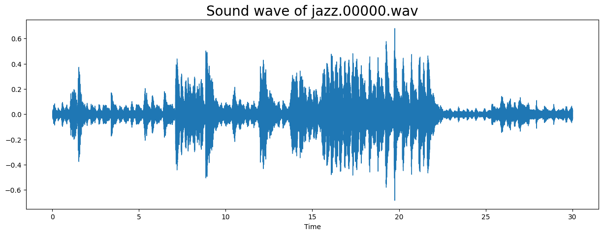
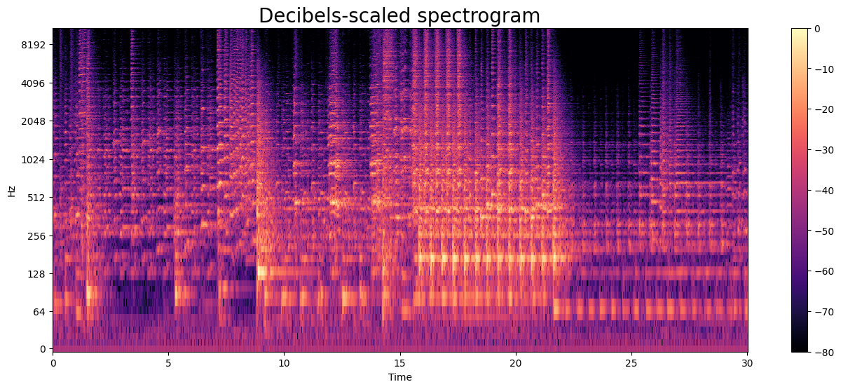
In this section we are looking at an example of an audio waveform. Then we’ll transform the sound wave to a spectrogram and compare it with the spectrogram that was included with the downloaded dataset.
# Inspect an audio file from the dataset.

sample_path = 'Data/genres_original/jazz/jazz.00000.wav'

# if you want to listen to the audio, uncomment below.
display.Audio(sample_path)
y, sample_rate = librosa.load(sample_path)

print('y:', y, '\n')
print('y shape:', np.shape(y), '\n')
print('Sample rate (KHz):', sample_rate, '\n')
print(f'Length of audio: {np.shape(y)[0]/sample_rate}')

# Plot th sound wave.

plt.figure(figsize=(15, 5))
librosa.display.waveshow(y=y, sr=sample_rate);
plt.title("Sound wave of jazz.00000.wav", fontsize=20)
plt.show()
y: [-0.00924683 -0.01177979 -0.01370239 ...  0.0071106   0.00561523
  0.00561523]

y shape: (661794,)

Sample rate (KHz): 22050

Length of audio: 30.013333333333332
# Convert sound wave to spectrogram.

# Short-time Fourier transform (STFT).

D = np.abs(librosa.stft(y, n_fft=2048, hop_length=512))
print('Shape of D object:', np.shape(D))

# Convert amplitude spectrogram to Decibels-scaled spectrogram.

DB = librosa.amplitude_to_db(D, ref = np.max)

# Creating the spectogram.

plt.figure(figsize = (16, 6))
librosa.display.specshow(DB, sr=sample_rate, hop_length=512,
                         x_axis='time', y_axis='log')
plt.colorbar()
plt.title('Decibels-scaled spectrogram', fontsize=20)
plt.show()
Shape of D object: (1025, 1293)
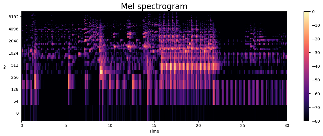
The mel spectrogram uses mel sclae intead of a linear one: mel scale is a perceptual scale of pitches judged by listeners to be equal in distance from one another. The reference point between this scale and normal frequency measurement is defined by assigning a perceptual pitch of 1000 mels to a 1000 Hz tone, 40 dB above the listener’s threshold. Above about 500 Hz, increasingly large intervals are judged by listeners to produce equal pitch increments.
# Convert sound wave to mel spectrogram.

y, sr = librosa.load(sample_path)

S = librosa.feature.melspectrogram(y=y, sr=sr)
S_DB = librosa.amplitude_to_db(S, ref=np.max)
plt.figure(figsize=(15, 5))
librosa.display.specshow(S_DB, sr=sr, hop_length=512,
                         x_axis='time', y_axis='log')
plt.colorbar()
plt.title("Mel spectrogram", fontsize=20)
plt.show()
# Visualize the mel spectrogram of the same sample from the dataset.

img_path = 'Data/images_original/jazz/jazz00000.png'
img = imageio.imread(img_path)
print(img.shape)

plt.imshow(img, interpolation='nearest')
plt.show()
(288, 432, 4)
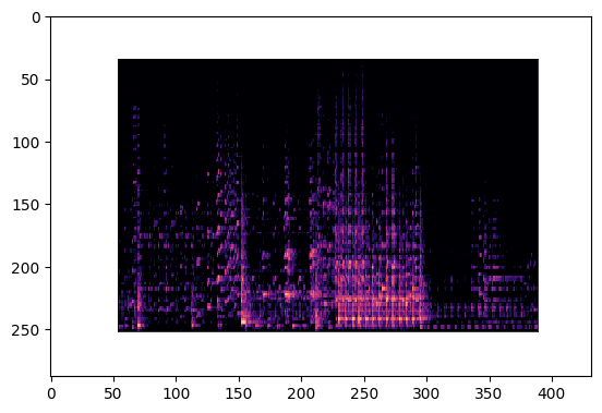
Train a simple CNN#
Helper functions (run me)#
Show code cell source
# @title Helper functions (run me)

def set_device():
  device = "cuda" if torch.cuda.is_available() else "cpu"
  if device != "cuda":
      print("WARNING: For this notebook to perform best, "
          "if possible, in the menu under `Runtime` -> "
          "`Change runtime type.`  select `GPU` ")
  else:
      print("GPU is enabled in this notebook.")

  return device


def plot_loss_accuracy(train_loss, train_acc, validation_loss, validation_acc):
  epochs = len(train_loss)
  fig, (ax1, ax2) = plt.subplots(1, 2)
  ax1.plot(list(range(epochs)), train_loss, label='Training Loss')
  ax1.plot(list(range(epochs)), validation_loss, label='Validation Loss')
  ax1.set_xlabel('Epochs')
  ax1.set_ylabel('Loss')
  ax1.set_title('Epoch vs Loss')
  ax1.legend()

  ax2.plot(list(range(epochs)), train_acc, label='Training Accuracy')
  ax2.plot(list(range(epochs)), validation_acc, label='Validation Accuracy')
  ax2.set_xlabel('Epochs')
  ax2.set_ylabel('Accuracy')
  ax2.set_title('Epoch vs Accuracy')
  ax2.legend()
  fig.set_size_inches(15.5, 5.5)
  plt.show()
device = set_device()
WARNING: For this notebook to perform best, if possible, in the menu under `Runtime` -> `Change runtime type.` select `GPU`
# Create folder with training, testing and validation data.

spectrograms_dir = "Data/images_original/"
folder_names = ['Data/train/', 'Data/test/', 'Data/val/']
train_dir = folder_names[0]
test_dir = folder_names[1]
val_dir = folder_names[2]

for f in folder_names:
  if os.path.exists(f):
    shutil.rmtree(f)
    os.mkdir(f)
  else:
    os.mkdir(f)

# Loop over all genres.

genres = list(os.listdir(spectrograms_dir))
for g in genres:
  # find all images & split in train, test, and validation
  src_file_paths= []
  for im in glob.glob(os.path.join(spectrograms_dir, f'{g}',"*.png"), recursive=True):
    src_file_paths.append(im)
  random.shuffle(src_file_paths)
  test_files = src_file_paths[0:10]
  val_files = src_file_paths[10:20]
  train_files = src_file_paths[20:]

  #  make destination folders for train and test images
  for f in folder_names:
    if not os.path.exists(os.path.join(f + f"{g}")):
      os.mkdir(os.path.join(f + f"{g}"))

  # copy training and testing images over
  for f in train_files:
    shutil.copy(f, os.path.join(os.path.join(train_dir + f"{g}") + '/',os.path.split(f)[1]))
  for f in test_files:
    shutil.copy(f, os.path.join(os.path.join(test_dir + f"{g}") + '/',os.path.split(f)[1]))
  for f in val_files:
    shutil.copy(f, os.path.join(os.path.join(val_dir + f"{g}") + '/',os.path.split(f)[1]))
# Data loading.

train_dataset = datasets.ImageFolder(
    train_dir,
    transforms.Compose([
        transforms.ToTensor(),
    ]))

train_loader = torch.utils.data.DataLoader(
    train_dataset, batch_size=25, shuffle=True, num_workers=0)

val_dataset = datasets.ImageFolder(
    val_dir,
    transforms.Compose([
        transforms.ToTensor(),
    ]))

val_loader = torch.utils.data.DataLoader(
    val_dataset, batch_size=25, shuffle=True, num_workers=0)
# Make a CNN & train it to predict genres.

class music_net(nn.Module):
  def __init__(self):
    """Intitalize neural net layers"""
    super(music_net, self).__init__()
    self.conv1 = nn.Conv2d(in_channels=3, out_channels=8, kernel_size=3, stride=1, padding=0)
    self.conv2 = nn.Conv2d(in_channels=8, out_channels=16, kernel_size=3, stride=1, padding=0)
    self.conv3 = nn.Conv2d(in_channels=16, out_channels=32, kernel_size=3, stride=1, padding=0)
    self.conv4 = nn.Conv2d(in_channels=32, out_channels=64, kernel_size=3, stride=1, padding=0)
    self.conv5 = nn.Conv2d(in_channels=64, out_channels=128, kernel_size=3, stride=1, padding=0)
    self.fc1 = nn.Linear(in_features=9856, out_features=10)

    self.batchnorm1 = nn.BatchNorm2d(num_features=8)
    self.batchnorm2 = nn.BatchNorm2d(num_features=16)
    self.batchnorm3 = nn.BatchNorm2d(num_features=32)
    self.batchnorm4 = nn.BatchNorm2d(num_features=64)
    self.batchnorm5 = nn.BatchNorm2d(num_features=128)

    self.dropout = nn.Dropout(p=0.3, inplace=False)


  def forward(self, x):
    # Conv layer 1.
    x = self.conv1(x)
    x = self.batchnorm1(x)
    x = F.relu(x)
    x = F.max_pool2d(x, kernel_size=2)

    # Conv layer 2.
    x = self.conv2(x)
    x = self.batchnorm2(x)
    x = F.relu(x)
    x = F.max_pool2d(x, kernel_size=2)

    # Conv layer 3.
    x = self.conv3(x)
    x = self.batchnorm3(x)
    x = F.relu(x)
    x = F.max_pool2d(x, kernel_size=2)

    # Conv layer 4.
    x = self.conv4(x)
    x = self.batchnorm4(x)
    x = F.relu(x)
    x = F.max_pool2d(x, kernel_size=2)

    # Conv layer 5.
    x = self.conv5(x)
    x = self.batchnorm5(x)
    x = F.relu(x)
    x = F.max_pool2d(x, kernel_size=2)

    # Fully connected layer 1.
    x = torch.flatten(x, 1)
    x = self.dropout(x)
    x = self.fc1(x)
    x = F.softmax(x)

    return x


def train(model, device, train_loader, validation_loader, epochs):
  criterion =  nn.CrossEntropyLoss()
  optimizer = torch.optim.Adam(model.parameters(), lr=0.0005)
  train_loss, validation_loss = [], []
  train_acc, validation_acc = [], []
  with tqdm(range(epochs), unit='epoch') as tepochs:
    tepochs.set_description('Training')
    for epoch in tepochs:
      model.train()
      # keep track of the running loss
      running_loss = 0.
      correct, total = 0, 0

      for data, target in train_loader:
        # getting the training set
        data, target = data.to(device), target.to(device)
        # Get the model output (call the model with the data from this batch)
        output = model(data)
        # Zero the gradients out)
        optimizer.zero_grad()
        # Get the Loss
        loss  = criterion(output, target)
        # Calculate the gradients
        loss.backward()
        # Update the weights (using the training step of the optimizer)
        optimizer.step()

        tepochs.set_postfix(loss=loss.item())
        running_loss += loss  # add the loss for this batch

        # get accuracy
        _, predicted = torch.max(output, 1)
        total += target.size(0)
        correct += (predicted == target).sum().item()

      # append the loss for this epoch
      train_loss.append(running_loss.detach().cpu().item()/len(train_loader))
      train_acc.append(correct/total)

      # evaluate on validation data
      model.eval()
      running_loss = 0.
      correct, total = 0, 0

      for data, target in validation_loader:
        # getting the validation set
        data, target = data.to(device), target.to(device)
        optimizer.zero_grad()
        output = model(data)
        loss = criterion(output, target)
        tepochs.set_postfix(loss=loss.item())
        running_loss += loss.item()
        # get accuracy
        _, predicted = torch.max(output, 1)
        total += target.size(0)
        correct += (predicted == target).sum().item()

      validation_loss.append(running_loss/len(validation_loader))
      validation_acc.append(correct/total)

  return train_loss, train_acc, validation_loss, validation_acc
# Run training.

net = music_net().to(device)
train_loss, train_acc, validation_loss, validation_acc = train(net, device, train_loader, val_loader, 50)

# Detach tensors from GPU
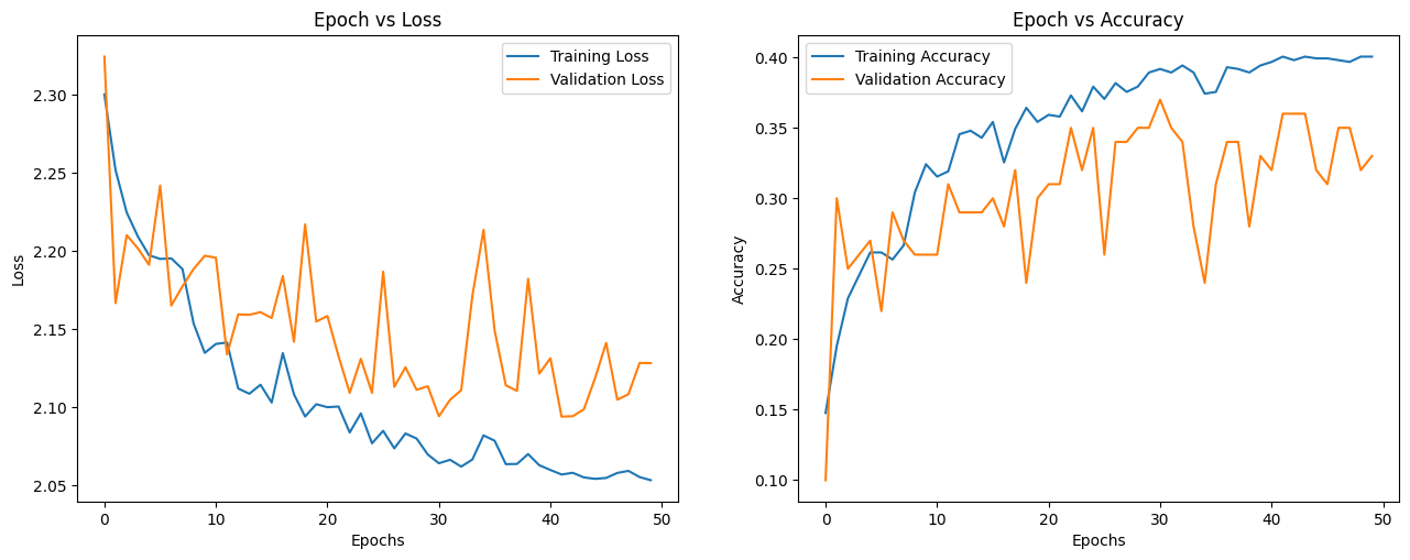
plot_loss_accuracy(train_loss, train_acc, validation_loss, validation_acc)
