![]()

Tutorial 2: Regularization techniques part 2#
Week 2, Day 1: Regularization
By Neuromatch Academy
Content creators: Ravi Teja Konkimalla, Mohitrajhu Lingan Kumaraian, Kevin Machado Gamboa, Kelson Shilling-Scrivo, Lyle Ungar
Content reviewers: Piyush Chauhan, Siwei Bai, Kelson Shilling-Scrivo, Jiaxin Cindy Tu
Content editors: Roberto Guidotti, Spiros Chavlis
Production editors: Saeed Salehi, Gagana B, Spiros Chavlis, Konstantine Tsafatinos
Tutorial Objectives#
Regularization as shrinkage of overparameterized models: L1 and L2
Regularization by Dropout
Regularization by Data Augmentation
Perils of Hyper-Parameter Tuning
Rethinking generalization
Setup#
Note that some of the code for today can take up to an hour to run. We have therefore “hidden” that code and shown the resulting outputs.
Install and import feedback gadget#
Show code cell source
# @title Install and import feedback gadget

!pip3 install vibecheck datatops --quiet

from vibecheck import DatatopsContentReviewContainer
def content_review(notebook_section: str):
    return DatatopsContentReviewContainer(
        "",  # No text prompt
        notebook_section,
        {
            "url": "https://pmyvdlilci.execute-api.us-east-1.amazonaws.com/klab",
            "name": "neuromatch_dl",
            "user_key": "f379rz8y",
        },
    ).render()


feedback_prefix = "W2D1_T2"
Uncomment to install dependencies#
Show code cell source
# @title Uncomment to install dependencies
# !pip install imageio --quiet
# !pip install imageio-ffmpeg --quiet
# Imports
import os
import copy
import torch
import random
import pathlib
import requests
from zipfile import ZipFile

import numpy as np
import matplotlib.pyplot as plt
import matplotlib.animation as animation

import torch.nn as nn
import torch.optim as optim
import torch.nn.functional as F

from torchvision import transforms
from torchvision.datasets import ImageFolder

from tqdm.auto import tqdm
from IPython.display import HTML, IFrame, YouTubeVideo, display
Figure Settings#
Show code cell source
# @title Figure Settings
import logging
logging.getLogger('matplotlib.font_manager').disabled = True

import ipywidgets as widgets
%matplotlib inline
%config InlineBackend.figure_format = 'retina'
plt.style.use("https://raw.githubusercontent.com/NeuromatchAcademy/content-creation/main/nma.mplstyle")
Loading Animal Faces Data#
Show code cell source
# @title Loading Animal Faces Data
print("Start downloading and unzipping `AnimalFaces` dataset...")
name = 'afhq'
fname = f"{name}.zip"
url = f"https://osf.io/kgfvj/download"

if not os.path.exists(fname):
  r = requests.get(url, allow_redirects=True)
  with open(fname, 'wb') as fh:
    fh.write(r.content)

  if os.path.exists(fname):
    with ZipFile(fname, 'r') as zfile:
      zfile.extractall(f".")
      os.remove(fname)

print("Download completed.")
Start downloading and unzipping `AnimalFaces` dataset...
Download completed.
Loading Animal Faces Randomized data#
Show code cell source
# @title Loading Animal Faces Randomized data

print("Start downloading and unzipping `Randomized AnimalFaces` dataset...")

names = ['afhq_random_32x32', 'afhq_10_32x32']
urls = ["https://osf.io/9sj7p/download",
        "https://osf.io/wvgkq/download"]


for i, name in enumerate(names):
  url = urls[i]
  fname = f"{name}.zip"

  if not os.path.exists(fname):
    r = requests.get(url, allow_redirects=True)
    with open(fname, 'wb') as fh:
      fh.write(r.content)

    if os.path.exists(fname):
      with ZipFile(fname, 'r') as zfile:
        zfile.extractall(f".")
        os.remove(fname)

print("Download completed.")
Start downloading and unzipping `Randomized AnimalFaces` dataset...
Download completed.
Plotting functions#
Show code cell source
# @title Plotting functions

def imshow(img):
  """
  Display unnormalized image

  Args:
    img: np.ndarray
      Datapoint to visualize

  Returns:
    Nothing
  """
  img = img / 2 + 0.5  # Unnormalize
  npimg = img.numpy()
  plt.imshow(np.transpose(npimg, (1, 2, 0)))
  plt.axis(False)
  plt.show()


def plot_weights(norm, labels, ws, title='Weight Size Measurement'):
  """
  Plot of weight size measurement [norm value vs layer]

  Args:
    norm: float
      Norm values
    labels: list
      Targets
    ws: list
      Weights
    title: string
      Title of plot

  Returns:
    Nothing
  """
  plt.figure(figsize=[8, 6])
  plt.title(title)
  plt.ylabel('Frobenius Norm Value')
  plt.xlabel('Model Layers')
  plt.bar(labels, ws)
  plt.axhline(y=norm,
              linewidth=1,
              color='r',
              ls='--',
              label='Total Model F-Norm')
  plt.legend()
  plt.show()


def visualize_data(dataloader):
  """
  Helper function to visualize data

  Args:
    dataloader: torch.tensor
      Dataloader to visualize

  Returns:
    Nothing
  """
  for idx, (data,label) in enumerate(dataloader):
    plt.figure(idx)
    # Choose the datapoint you would like to visualize
    index = 22

    # Choose that datapoint using index and permute the dimensions
    # and bring the pixel values between [0,1]
    data = data[index].permute(1, 2, 0) * \
           torch.tensor([0.5, 0.5, 0.5]) + \
           torch.tensor([0.5, 0.5, 0.5])

    # Convert the torch tensor into numpy
    data = data.numpy()

    plt.imshow(data)
    plt.axis(False)
    image_class = classes[label[index].item()]
    print(f'The image belongs to : {image_class}')

  plt.show()
Helper functions#
Show code cell source
# @title Helper functions

class AnimalNet(nn.Module):
  """
  Network Class - Animal Faces with following structure:
  nn.Linear(3 * 32 * 32, 128) # Fully connected layer 1
  nn.Linear(128, 32) # Fully connected layer 2
  nn.Linear(32, 3) # Fully connected layer 3
  """

  def __init__(self):
    """
    Initialize parameters of AnimalNet

    Args:
      None

    Returns:
      Nothing
    """
    super(AnimalNet, self).__init__()
    self.fc1 = nn.Linear(3 * 32 * 32, 128)
    self.fc2 = nn.Linear(128, 32)
    self.fc3 = nn.Linear(32, 3)

  def forward(self, x):
    """
    Forward Pass of AnimalNet

    Args:
      x: torch.tensor
        Input features

    Returns:
      output: torch.tensor
        Outputs/Predictions
    """
    x = x.view(x.shape[0], -1)
    x = F.relu(self.fc1(x))
    x = F.relu(self.fc2(x))
    x = self.fc3(x)
    output = F.log_softmax(x, dim=1)
    return output


class Net(nn.Module):
  """
  Network Class - 2D with following structure
  nn.Linear(1, 300) + leaky_relu(self.fc1(x)) # First fully connected layer
  nn.Linear(300, 500) + leaky_relu(self.fc2(x)) # Second fully connected layer
  nn.Linear(500, 1) # Final fully connected layer
  """

  def __init__(self):
    """
    Initialize parameters of Net

    Args:
      None

    Returns:
      Nothing
    """
    super(Net, self).__init__()

    self.fc1 = nn.Linear(1, 300)
    self.fc2 = nn.Linear(300, 500)
    self.fc3 = nn.Linear(500, 1)

  def forward(self, x):
    """
    Forward pass of Net

    Args:
      x: torch.tensor
        Input features

    Returns:
      x: torch.tensor
        Output/Predictions
    """
    x = F.leaky_relu(self.fc1(x))
    x = F.leaky_relu(self.fc2(x))
    output = self.fc3(x)
    return output


class BigAnimalNet(nn.Module):
  """
  Network Class - Animal Faces with following structure:
  nn.Linear(3*32*32, 124) + leaky_relu(self.fc1(x)) # First fully connected layer
  nn.Linear(124, 64) + leaky_relu(self.fc2(x)) # Second fully connected layer
  nn.Linear(64, 3) # Final fully connected layer
  """

  def __init__(self):
    """
    Initialize parameters for BigAnimalNet

    Args:
      None

    Returns:
      Nothing
    """
    super(BigAnimalNet, self).__init__()
    self.fc1 = nn.Linear(3*32*32, 124)
    self.fc2 = nn.Linear(124, 64)
    self.fc3 = nn.Linear(64, 3)

  def forward(self, x):
    """
    Forward pass of BigAnimalNet

    Args:
      x: torch.tensor
        Input features

    Returns:
      x: torch.tensor
        Output/Predictions
    """
    x = x.view(x.shape[0],-1)
    x = F.leaky_relu(self.fc1(x))
    x = F.leaky_relu(self.fc2(x))
    x = self.fc3(x)
    output = F.log_softmax(x, dim=1)
    return output


def train(args, model, train_loader, optimizer, epoch,
          reg_function1=None, reg_function2=None, criterion=F.nll_loss):
  """
  Trains the current input model using the data
  from Train_loader and Updates parameters for a single pass

  Args:
    args: dictionary
      Dictionary with epochs: 200, lr: 5e-3, momentum: 0.9, device: DEVICE
    model: nn.module
      Neural network instance
    train_loader: torch.loader
      Input dataset
    optimizer: function
      Optimizer
    reg_function1: function
      Regularisation function [default: None]
    reg_function2: function
      Regularisation function [default: None]
    criterion: function
      Specifies loss function [default: nll_loss]

  Returns:
    model: nn.module
      Neural network instance post training
  """
  device = args['device']
  model.train()
  for batch_idx, (data, target) in enumerate(train_loader):
    data, target = data.to(device), target.to(device)
    optimizer.zero_grad()
    output = model(data)
    # L1 regularization
    if reg_function2 is None and reg_function1 is not None:
      loss = criterion(output, target) + args['lambda1']*reg_function1(model)
    # L2 regularization
    elif reg_function1 is None and reg_function2 is not None:
      loss = criterion(output, target) + args['lambda2']*reg_function2(model)
    # No regularization
    elif reg_function1 is None and reg_function2 is None:
      loss = criterion(output, target)
    # Both L1 and L2 regularizations
    else:
      loss = criterion(output, target) + args['lambda1']*reg_function1(model) + args['lambda2']*reg_function2(model)
    loss.backward()
    optimizer.step()

  return model


def test(model, test_loader, loader='Test', criterion=F.nll_loss,
         device='cpu'):
  """
  Tests the current model

  Args:
    model: nn.module
      Neural network instance
    device: string
      GPU/CUDA if available, CPU otherwise
    test_loader: torch.loader
      Test dataset
    criterion: function
      Specifies loss function [default: nll_loss]

  Returns:
    test_loss: float
      Test loss
  """
  model.eval()
  test_loss = 0
  correct = 0
  with torch.no_grad():
    for data, target in test_loader:
      data, target = data.to(device), target.to(device)
      output = model(data)
      test_loss += criterion(output, target, reduction='sum').item()  # sum up batch loss
      pred = output.argmax(dim=1, keepdim=True)  # Get the index of the max log-probability
      correct += pred.eq(target.view_as(pred)).sum().item()

  test_loss /= len(test_loader.dataset)
  return 100. * correct / len(test_loader.dataset)


def main(args, model, train_loader, val_loader, test_data,
         reg_function1=None, reg_function2=None, criterion=F.nll_loss):
  """
  Trains the model with train_loader and
  tests the learned model using val_loader

  Args:
    args: dictionary
      Dictionary with epochs: 200, lr: 5e-3, momentum: 0.9, device: DEVICE
    model: nn.module
      Neural network instance
    train_loader: torch.loader
      Train dataset
    val_loader: torch.loader
      Validation set
    reg_function1: function
      Regularisation function [default: None]
    reg_function2: function
      Regularisation function [default: None]

  Returns:
    val_acc_list: list
      Log of validation accuracy
    train_acc_list: list
      Log of training accuracy
    param_norm_list: list
      Log of frobenius norm
    trained_model: nn.module
      Trained model/model post training
  """
  device = args['device']

  model = model.to(device)
  optimizer = optim.SGD(model.parameters(), lr=args['lr'], momentum=args['momentum'])

  val_acc_list, train_acc_list,param_norm_list = [], [], []
  for epoch in tqdm(range(args['epochs'])):
    trained_model = train(args, model, train_loader, optimizer, epoch,
                          reg_function1=reg_function1,
                          reg_function2=reg_function2)
    train_acc = test(trained_model, train_loader, loader='Train', device=device)
    val_acc = test(trained_model, val_loader, loader='Val', device=device)
    param_norm = calculate_frobenius_norm(trained_model)
    train_acc_list.append(train_acc)
    val_acc_list.append(val_acc)
    param_norm_list.append(param_norm)

  return val_acc_list, train_acc_list, param_norm_list, model


def calculate_frobenius_norm(model):
    """
    Function to calculate frobenius norm

    Args:
      model: nn.module
        Neural network instance

    Returns:
      norm: float
        Frobenius norm
    """
    norm = 0.0
    # Sum the square of all parameters
    for name,param in model.named_parameters():
        norm += torch.norm(param).data**2
    # Return a square root of the sum of squares of all the parameters
    return norm**0.5


def early_stopping_main(args, model, train_loader, val_loader, test_data):
  """
  Function to simulate early stopping

  Args:
    args: dictionary
      Dictionary with epochs: 200, lr: 5e-3, momentum: 0.9, device: DEVICE
    model: nn.module
      Neural network instance
    train_loader: torch.loader
      Train dataset
    val_loader: torch.loader
      Validation set

  Returns:
    val_acc_list: list
      Val accuracy log until early stop point
    train_acc_list: list
      Training accuracy log until early stop point
    best_model: nn.module
      Model performing best with early stopping
    best_epoch: int
      Epoch at which early stopping occurs
  """
  device = args['device']

  model = model.to(device)
  optimizer = optim.SGD(model.parameters(), lr=args['lr'], momentum=args['momentum'])

  best_acc  = 0.0
  best_epoch = 0

  # Number of successive epochs that you want to wait before stopping training process
  patience = 20

  # Keps track of number of epochs during which the val_acc was less than best_acc
  wait = 0

  val_acc_list, train_acc_list = [], []
  for epoch in tqdm(range(args['epochs'])):
    trained_model = train(args, model, device, train_loader, optimizer, epoch)
    train_acc = test(trained_model, train_loader, loader='Train', device=device)
    val_acc = test(trained_model, val_loader, loader='Val', device=device)
    if (val_acc > best_acc):
      best_acc = val_acc
      best_epoch = epoch
      best_model = copy.deepcopy(trained_model)
      wait = 0
    else:
      wait += 1
    if (wait > patience):
      print(f'Early stopped on epoch: {epoch}')
      break
    train_acc_list.append(train_acc)
    val_acc_list.append(val_acc)

  return val_acc_list, train_acc_list, best_model, best_epoch
Set random seed#
Executing set_seed(seed=seed) you are setting the seed
Show code cell source
# @title Set random seed
# @markdown Executing `set_seed(seed=seed)` you are setting the seed

# For DL its critical to set the random seed so that students can have a
# baseline to compare their results to expected results.
# Read more here: https://pytorch.org/docs/stable/notes/randomness.html

# Call `set_seed` function in the exercises to ensure reproducibility.
def set_seed(seed=None, seed_torch=True):
  """
  Function that controls randomness. NumPy and random modules must be imported.

  Args:
    seed : Integer
      A non-negative integer that defines the random state. Default is `None`.
    seed_torch : Boolean
      If `True` sets the random seed for pytorch tensors, so pytorch module
      must be imported. Default is `True`.

  Returns:
    Nothing.
  """
  if seed is None:
    seed = np.random.choice(2 ** 32)
  random.seed(seed)
  np.random.seed(seed)
  if seed_torch:
    torch.manual_seed(seed)
    torch.cuda.manual_seed_all(seed)
    torch.cuda.manual_seed(seed)
    torch.backends.cudnn.benchmark = False
    torch.backends.cudnn.deterministic = True

  print(f'Random seed {seed} has been set.')


# In case that `DataLoader` is used
def seed_worker(worker_id):
  """
  DataLoader will reseed workers following randomness in
  multi-process data loading algorithm.

  Args:
    worker_id: integer
      ID of subprocess to seed. 0 means that
      the data will be loaded in the main process
      Refer: https://pytorch.org/docs/stable/data.html#data-loading-randomness for more details

  Returns:
    Nothing
  """
  worker_seed = torch.initial_seed() % 2**32
  np.random.seed(worker_seed)
  random.seed(worker_seed)
Set device (GPU or CPU). Execute set_device()#
Show code cell source
# @title Set device (GPU or CPU). Execute `set_device()`
# especially if torch modules used.

# Inform the user if the notebook uses GPU or CPU.

def set_device():
  """
  Set the device. CUDA if available, CPU otherwise

  Args:
    None

  Returns:
    Nothing
  """
  device = "cuda" if torch.cuda.is_available() else "cpu"
  if device != "cuda":
    print("WARNING: For this notebook to perform best, "
        "if possible, in the menu under `Runtime` -> "
        "`Change runtime type.`  select `GPU` ")
  else:
    print("GPU is enabled in this notebook.")

  return device
SEED = 2021
set_seed(seed=SEED)
DEVICE = set_device()
Random seed 2021 has been set.
WARNING: For this notebook to perform best, if possible, in the menu under `Runtime` -> `Change runtime type.`  select `GPU`
Dataloaders for the Dataset#
Show code cell source
# @title Dataloaders for the Dataset
## Dataloaders for the Dataset
batch_size = 128
classes = ('cat', 'dog', 'wild')

train_transform = transforms.Compose([
     transforms.ToTensor(),
     transforms.Normalize((0.5, 0.5, 0.5), (0.5, 0.5, 0.5))
     ])
data_path = pathlib.Path('.')/'afhq' # Using pathlib to be compatible with all OS's
img_dataset = ImageFolder(data_path/'train', transform=train_transform)


####################################################
g_seed = torch.Generator()
g_seed.manual_seed(SEED)


## Dataloaders for the  Original Dataset
img_train_data, img_val_data,_ = torch.utils.data.random_split(img_dataset,
                                                               [100, 100, 14430])

# Creating train_loader and Val_loader
train_loader = torch.utils.data.DataLoader(img_train_data,
                                           batch_size=batch_size,
                                           worker_init_fn=seed_worker,
                                           num_workers=2,
                                           generator=g_seed)
val_loader = torch.utils.data.DataLoader(img_val_data,
                                         batch_size=1000,
                                         num_workers=2,
                                         worker_init_fn=seed_worker,
                                         generator=g_seed)

# Creating test dataset
test_transform = transforms.Compose([
     transforms.ToTensor(),
     transforms.Normalize((0.5, 0.5, 0.5), (0.5, 0.5, 0.5))
     ])
img_test_dataset = ImageFolder(data_path/'val', transform=test_transform)


####################################################

## Dataloaders for the  Random Dataset

# Splitting randomized data into training and validation data
data_path = pathlib.Path('.')/'afhq_random_32x32/afhq_random' # using pathlib to be compatible with all OS's
img_dataset = ImageFolder(data_path/'train', transform=train_transform)
random_img_train_data, random_img_val_data,_ = torch.utils.data.random_split(img_dataset, [100,100,14430])

# Randomized train and validation dataloader
rand_train_loader = torch.utils.data.DataLoader(random_img_train_data,
                                                batch_size=batch_size,
                                                num_workers=2,
                                                worker_init_fn=seed_worker,
                                                generator=g_seed)
rand_val_loader = torch.utils.data.DataLoader(random_img_val_data,
                                              batch_size=1000,
                                              num_workers=2,
                                              worker_init_fn=seed_worker,
                                              generator=g_seed)

####################################################

## Dataloaders for the Partially Random Dataset

# Splitting data between training and validation dataset for partially randomized data
data_path = pathlib.Path('.')/'afhq_10_32x32/afhq_10' # using pathlib to be compatible with all OS's
img_dataset = ImageFolder(data_path/'train', transform=train_transform)
partially_random_train_data, partially_random_val_data, _ = torch.utils.data.random_split(img_dataset, [100,100,14430])

# Training and Validation loader for partially randomized data
partial_rand_train_loader = torch.utils.data.DataLoader(partially_random_train_data,
                                                        batch_size=batch_size,
                                                        num_workers=2,
                                                        worker_init_fn=seed_worker,
                                                        generator=g_seed)
partial_rand_val_loader = torch.utils.data.DataLoader(partially_random_val_data,
                                                      batch_size=1000,
                                                      num_workers=2,
                                                      worker_init_fn=seed_worker,
                                                      generator=g_seed)
Section 1: L1 and L2 Regularization#
Time estimate: ~30 mins
Video 1: L1 and L2 regularization#
Submit your feedback#
Show code cell source
# @title Submit your feedback
content_review(f"{feedback_prefix}_L1_and_L2_regularization_Video")
Some of you might have already come across L1 and L2 regularization before in other courses. L1 and L2 are the most common types of regularization. These update the general cost function by adding another term known as the regularization term.
This regularization term makes the parameters smaller, giving simpler models that will overfit less.
Discuss among your teammates whether the above assumption is good or bad?
Section 1.1: Unregularized Model#
Dataloaders for Regularization#
Show code cell source
# @markdown #### Dataloaders for Regularization
data_path = pathlib.Path('.')/'afhq' # Using pathlib to be compatible with all OS's
img_dataset = ImageFolder(data_path/'train', transform=train_transform)

# Splitting dataset
reg_train_data, reg_val_data,_ = torch.utils.data.random_split(img_dataset,
                                                               [30, 100, 14500])
g_seed = torch.Generator()
g_seed.manual_seed(SEED)

# Creating train_loader and Val_loader
reg_train_loader = torch.utils.data.DataLoader(reg_train_data,
                                               batch_size=batch_size,
                                               worker_init_fn=seed_worker,
                                               num_workers=2,
                                               generator=g_seed)
reg_val_loader = torch.utils.data.DataLoader(reg_val_data,
                                             batch_size=1000,
                                             worker_init_fn=seed_worker,
                                             num_workers=2,
                                             generator=g_seed)
Now let’s train a model without regularization and keep it aside as our benchmark for this section.
# Set the arguments
args = {
    'epochs': 150,
    'lr': 5e-3,
    'momentum': 0.99,
    'device': DEVICE,
}

# Initialize the model
set_seed(seed=SEED)
model = AnimalNet()

# Train the model
val_acc_unreg, train_acc_unreg, param_norm_unreg, _ = main(args,
                                                           model,
                                                           reg_train_loader,
                                                           reg_val_loader,
                                                           img_test_dataset)

# Train and Test accuracy plot
plt.figure()
plt.plot(val_acc_unreg, label='Val Accuracy', c='red', ls='dashed')
plt.plot(train_acc_unreg, label='Train Accuracy', c='red', ls='solid')
plt.axhline(y=max(val_acc_unreg), c='green', ls='dashed')
plt.title('Unregularized Model')
plt.ylabel('Accuracy (%)')
plt.xlabel('Epoch')
plt.legend()
plt.show()
print(f"Maximum Validation Accuracy reached: {max(val_acc_unreg)}")
Random seed 2021 has been set.
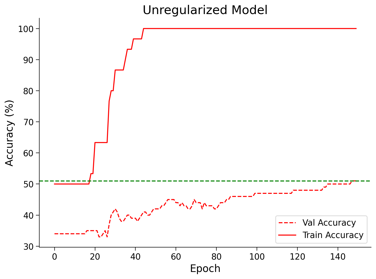
Maximum Validation Accuracy reached: 51.0
Section 1.2: L1 Regularization#
L1 Regularization (or LASSO\(^{\ddagger}\)) uses a penalty which is the sum of the absolute value of all the weights in the Deep Learning architecture, resulting in the following loss function (\(L\) is the usual Cross-Entropy loss):
where \(r\) denotes the layer, and \(ij\) the specific weight in that layer.
At a high level, L1 Regularization is similar to L2 Regularization since it leads to smaller weights (you will see the analogy in the next subsection). It results in the following weight update equation when using Stochastic Gradient Descent:
where \(\text{sgn}(\cdot)\) is the sign function, such that
\(^{\ddagger}\)LASSO: Least Absolute Shrinkage and Selection Operator
Coding Exercise 1.1: L1 Regularization#
Write a function that calculates the L1 norm of all the tensors of a PyTorch model.
def l1_reg(model):
  """
  This function calculates the l1 norm of the all the tensors in the model

  Args:
    model: nn.module
      Neural network instance

  Returns:
    l1: float
      L1 norm of the all the tensors in the model
  """
  l1 = 0.0
  ####################################################################
  # Fill in all missing code below (...),
  # then remove or comment the line below to test your function
  raise NotImplementedError("Complete the l1_reg function")
  ####################################################################
  for param in model.parameters():
    l1 += ...

  return l1


set_seed(seed=SEED)
## uncomment to test
# net = nn.Linear(20, 20)
# print(f"L1 norm of the model: {l1_reg(net)}")
Random seed 2021 has been set.
Random seed 2021 has been set.
L1 norm of the model: 48.445133209228516
Submit your feedback#
Show code cell source
# @title Submit your feedback
content_review(f"{feedback_prefix}_L1_regularization_Exercise")
Now, let’s train a classifier that uses L1 regularization. Tune the hyperparameter lambda1 such that the validation accuracy is higher than that of the unregularized model.
# Set the arguments
args1 = {
    'test_batch_size': 1000,
    'epochs': 150,
    'lr': 5e-3,
    'momentum': 0.99,
    'device': DEVICE,
    'lambda1': 0.001  # <<<<<<<< Tune the hyperparameter lambda1
}

# Initialize the model
set_seed(seed=SEED)
model = AnimalNet()

# Train the model
val_acc_l1reg, train_acc_l1reg, param_norm_l1reg, _ = main(args1,
                                                           model,
                                                           reg_train_loader,
                                                           reg_val_loader,
                                                           img_test_dataset,
                                                           reg_function1=l1_reg)

# Train and Test accuracy plot
plt.figure()
plt.plot(val_acc_l1reg, label='Val Accuracy L1 Regularized',
         c='red', ls='dashed')
plt.plot(train_acc_l1reg, label='Train Accuracy L1 regularized',
         c='red', ls='solid')
plt.axhline(y=max(val_acc_l1reg), c='green', ls='dashed')
plt.title('L1 regularized model')
plt.ylabel('Accuracy (%)')
plt.xlabel('Epoch')
plt.legend()
plt.show()
print(f"Maximum Validation Accuracy Reached: {max(val_acc_l1reg)}")
What value of lambda1 hyperparameter worked for L1 Regularization?
Note: that the \(\lambda\) in the equations is the lambda1 in the code for clarity.
Submit your feedback#
Show code cell source
# @title Submit your feedback
content_review(f"{feedback_prefix}_Tune_lambda1_Exercise")
Section 1.3: L2 / Ridge Regularization#
L2 Regularization (or Ridge), also referred to as “Weight Decay”, is widely used. It works by adding a quadratic penalty term to the Cross-Entropy Loss Function \(L\), which results in a new Loss Function \(L_R\) given by:
where, again, \(r\) superscript denotes the layer, and \(ij\) the specific weight in that layer.
To get further insight into L2 Regularization, we investigate its effect on the Gradient Descent based update equations for the weight and bias parameters. Taking the derivative on both sides of the above equation, we obtain
Thus the weight update rule becomes:
where \(\eta\) is the learning rate.
Coding Exercise 1.2: L2 Regularization#
Write a function that calculates the L2 norm of all the tensors of a PyTorch model. (What did we call this before?)
def l2_reg(model):
  """
  This function calculates the l2 norm of the all the tensors in the model

  Args:
    model: nn.module
      Neural network instance

  Returns:
    l2: float
      L2 norm of the all the tensors in the model
  """

  l2 = 0.0
  ####################################################################
  # Fill in all missing code below (...),
  # then remove or comment the line below to test your function
  raise NotImplementedError("Complete the l2_reg function")
  ####################################################################
  for param in model.parameters():
    l2 += ...

  return l2


set_seed(SEED)
## uncomment to test
# net = nn.Linear(20, 20)
# print(f"L2 norm of the model: {l2_reg(net)}")
Random seed 2021 has been set.
Random seed 2021 has been set.
L2 norm of the model: 7.328375816345215
Submit your feedback#
Show code cell source
# @title Submit your feedback
content_review(f"{feedback_prefix}_L2_Ridge_Regularization_Exercise")
Now we’ll train a classifier that uses L2 regularization. Tune the hyperparameter lambda2 such that the validation accuracy is higher than that of the unregularized model.
# Set the arguments
args2 = {
    'test_batch_size': 1000,
    'epochs': 150,
    'lr': 5e-3,
    'momentum': 0.99,
    'device': DEVICE,
    'lambda2': 0.001  # <<<<<<<< Tune the hyperparameter lambda2
}

# Initialize the model
set_seed(seed=SEED)
model = AnimalNet()

# Train the model
val_acc_l2reg, train_acc_l2reg, param_norm_l2reg, model = main(args2,
                                                               model,
                                                               train_loader,
                                                               val_loader,
                                                               img_test_dataset,
                                                               reg_function2=l2_reg)

## Train and Test accuracy plot
plt.figure()
plt.plot(val_acc_l2reg, label='Val Accuracy L2 regularized',
         c='red', ls='dashed')
plt.plot(train_acc_l2reg, label='Train Accuracy L2 regularized',
         c='red', ls='solid')
plt.axhline(y=max(val_acc_l2reg), c='green', ls='dashed')
plt.title('L2 Regularized Model')
plt.ylabel('Accuracy (%)')
plt.xlabel('Epoch')
plt.legend()
plt.show()
print(f"Maximum Validation Accuracy reached: {max(val_acc_l2reg)}")
What value lambda2 worked for L2 Regularization?
Note: that the \(\lambda\) in the equations is the lambda2 in the code for clarity.
Submit your feedback#
Show code cell source
# @title Submit your feedback
content_review(f"{feedback_prefix}_Tune_lambda2_Exercise")
Now, let’s run a model with both L1 and L2 regularization terms.
Show code cell source
# @markdown Visualize all of them together (Run Me!)

# @markdown `lambda1=0.001` and `lambda2=0.001`

args3 = {
    'test_batch_size': 1000,
    'epochs': 150,
    'lr': 5e-3,
    'momentum': 0.99,
    'device': DEVICE,
    'lambda1': 0.001,
    'lambda2': 0.001
}

# Initialize the model
set_seed(seed=SEED)
model = AnimalNet()
val_acc_l1l2reg, train_acc_l1l2reg, param_norm_l1l2reg, _ = main(args3,
                                                                 model,
                                                                 train_loader,
                                                                 val_loader,
                                                                 img_test_dataset,
                                                                 reg_function1=l1_reg,
                                                                 reg_function2=l2_reg)

plt.figure()

plt.plot(val_acc_l2reg, c='red', ls='dashed')
plt.plot(train_acc_l2reg,
         label=f"L2 regularized, $\lambda_2$={args2['lambda2']}",
         c='red', ls='solid')
plt.axhline(y=max(val_acc_l2reg), c='red', ls='dashed')

plt.plot(val_acc_l1reg, c='green', ls = 'dashed')
plt.plot(train_acc_l1reg,
         label=f"L1 regularized, $\lambda_1$={args1['lambda1']}",
         c='green', ls='solid')
plt.axhline(y=max(val_acc_l1reg), c='green', ls='dashed')

plt.plot(val_acc_unreg, c='blue', ls = 'dashed')
plt.plot(train_acc_unreg,
         label='Unregularized', c='blue', ls='solid')
plt.axhline(y=max(val_acc_unreg), c='blue', ls='dashed')

plt.plot(val_acc_l1l2reg, c='orange', ls='dashed')
plt.plot(train_acc_l1l2reg,
         label=f"L1+L2 regularized, $\lambda_1$={args3['lambda1']}, $\lambda_2$={args3['lambda2']}",
         c='orange', ls='solid')
plt.axhline(y=max(val_acc_l1l2reg), c='orange', ls = 'dashed')

plt.xlabel('Epoch')
plt.ylabel('Accuracy (%)')
plt.legend()
plt.show()
Now, let’s visualize what these different regularizations do to the model’s parameters. We observe the effect by computing the size (technically, the Frobenius norm).
x =  param_norm_unreg[0]
print(x)
tensor(7.3810)
Visualize Norm of the Models (Train Me!)#
Show code cell source
# @markdown #### Visualize Norm of the Models (Train Me!)
plt.figure()
plt.plot([i.cpu().numpy() for i in param_norm_unreg],
         label='Unregularized', c='blue')
plt.plot([i.cpu().numpy() for i in param_norm_l1reg],
         label='L1 Regularized', c='green')
plt.plot([i.cpu().numpy() for i in param_norm_l2reg],
         label='L2 Regularized', c='red')
plt.plot([i.cpu().numpy() for i in param_norm_l1l2reg],
         label='L1+L2 Regularized', c='orange')
plt.xlabel('Epoch')
plt.ylabel('Parameter Norms')
plt.legend()
plt.show()
In the above plots, you should have seen that the validation accuracies fluctuate even after the model achieves 100% train accuracy. Thus, the model is still trying to learn something. Why would this be the case?
Section 2: Dropout#
Time estimate: ~25 mins
Video 2: Dropout#
Submit your feedback#
Show code cell source
# @title Submit your feedback
content_review(f"{feedback_prefix}_Dropout_Video")
With Dropout, we literally drop out (zero out) some neurons during training. Throughout the training, the standard dropout zeros out some fraction (usually 50%) of the nodes in each layer, and on each iteration, before calculating the subsequent layer. Randomly selecting different subsets to drop out introduces noise into the process and reduces overfitting.

Now let’s revisit the toy dataset we generated above to visualize how the Dropout stabilizes training on a noisy dataset. We will slightly modify the architecture we used above to add dropout layers.
class NetDropout(nn.Module):
  """
  Network Class - 2D with the following structure:
  nn.Linear(1, 300) + leaky_relu(self.dropout1(self.fc1(x))) # First fully connected layer with 0.4 dropout
  nn.Linear(300, 500) + leaky_relu(self.dropout2(self.fc2(x))) # Second fully connected layer with 0.2 dropout
  nn.Linear(500, 1) # Final fully connected layer
  """

  def __init__(self):
    """
    Initialize parameters of NetDropout

    Args:
      None

    Returns:
      Nothing
    """
    super(NetDropout, self).__init__()

    self.fc1 = nn.Linear(1, 300)
    self.fc2 = nn.Linear(300, 500)
    self.fc3 = nn.Linear(500, 1)
    # We add two dropout layers
    self.dropout1 = nn.Dropout(0.4)
    self.dropout2 = nn.Dropout(0.2)

  def forward(self, x):
    """
    Forward pass of NetDropout

    Args:
      x: torch.tensor
        Input features

    Returns:
      output: torch.tensor
        Output/Predictions
    """
    x = F.leaky_relu(self.dropout1(self.fc1(x)))
    x = F.leaky_relu(self.dropout2(self.fc2(x)))
    output = self.fc3(x)
    return output
Run to train the default network#
Show code cell source
# @markdown #### Run to train the default network
set_seed(seed=SEED)

# Creating train data
X = torch.rand((10, 1))
X.sort(dim = 0)
Y = 2*X + 2*torch.empty((X.shape[0], 1)).normal_(mean=0, std=1)  # adding small error in the data

X = X.unsqueeze_(1)
Y = Y.unsqueeze_(1)

# Creating test dataset
X_test = torch.linspace(0, 1, 40)
X_test = X_test.reshape((40, 1, 1))

# Train the network on toy dataset
model = Net()
criterion = nn.MSELoss()
optimizer = optim.Adam(model.parameters(), lr=1e-4)
max_epochs = 10000
iters = 0

running_predictions = np.empty((40, (int)(max_epochs/500 + 1)))

train_loss = []
test_loss = []
model_norm = []

for epoch in tqdm(range(max_epochs)):

  # Training
  model_norm.append(calculate_frobenius_norm(model))
  model.train()
  optimizer.zero_grad()
  predictions = model(X)
  loss = criterion(predictions,Y)
  loss.backward()
  optimizer.step()

  train_loss.append(loss.data)
  model.eval()
  Y_test = model(X_test)
  loss = criterion(Y_test, 2*X_test)
  test_loss.append(loss.data)

  if (epoch % 500 == 0 or epoch == max_epochs - 1):
    running_predictions[:, iters] = Y_test[:, 0, 0].detach().numpy()
    iters += 1
Random seed 2021 has been set.
# Train the network on toy dataset

# Initialize the model
set_seed(seed=SEED)
model = NetDropout()
criterion = nn.MSELoss()
optimizer = optim.Adam(model.parameters(), lr=1e-4)
max_epochs = 10000
iters = 0

running_predictions_dp = np.empty((40, (int)(max_epochs / 500)))

train_loss_dp = []
test_loss_dp = []
model_norm_dp = []

for epoch in tqdm(range(max_epochs)):

  # Training
  model_norm_dp.append(calculate_frobenius_norm(model))
  model.train()
  optimizer.zero_grad()
  predictions = model(X)
  loss = criterion(predictions, Y)
  loss.backward()
  optimizer.step()

  train_loss_dp.append(loss.data)
  model.eval()
  Y_test = model(X_test)
  loss = criterion(Y_test, 2*X_test)
  test_loss_dp.append(loss.data)

  if (epoch % 500 == 0 or epoch == max_epochs):
    running_predictions_dp[:, iters] = Y_test[:, 0, 0].detach().numpy()
    iters += 1
Random seed 2021 has been set.
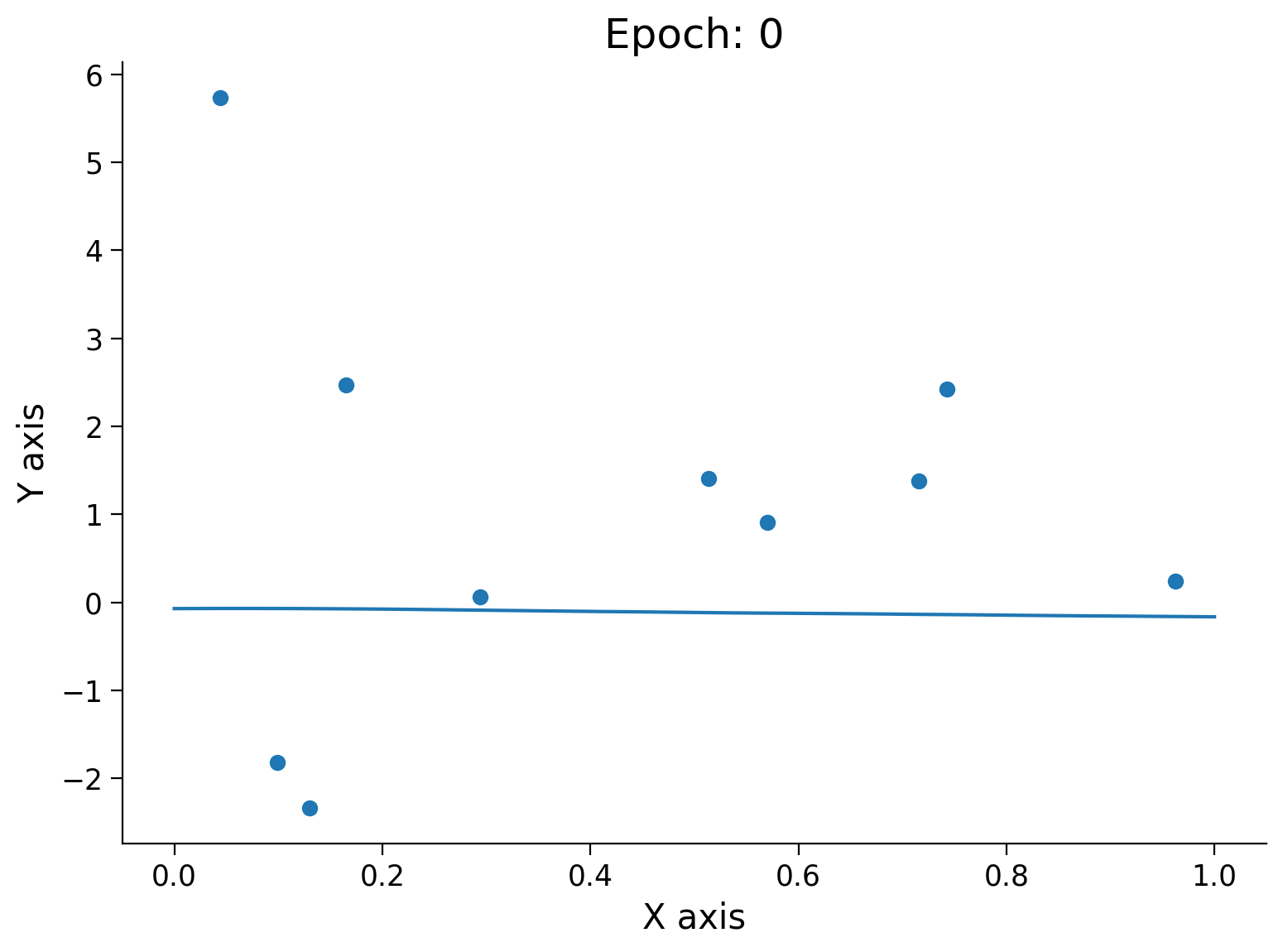
Now that we have finished the training, let’s see how the model has evolved over the training process.
Animation! (Run Me!)
Show code cell source
# @markdown Animation! (Run Me!)
set_seed(seed=SEED)

fig = plt.figure(figsize=(8, 6))
ax = plt.axes()

def frame(i):
  ax.clear()
  ax.scatter(X[:, 0, :].numpy(), Y[:, 0, :].numpy())
  plot = ax.plot(X_test[:, 0, :].detach().numpy(),
                 running_predictions_dp[:, i])
  title = f"Epoch: {i*500}"
  plt.title(title)
  ax.set_xlabel("X axis")
  ax.set_ylabel("Y axis")
  return plot


anim = animation.FuncAnimation(fig, frame, frames=range(20),
                               blit=False, repeat=False,
                               repeat_delay=10000)
html_anim = HTML(anim.to_html5_video());
plt.close()
display(html_anim)
Random seed 2021 has been set.
---------------------------------------------------------------------------
RuntimeError                              Traceback (most recent call last)
Cell In[34], line 22
     16   return plot
     19 anim = animation.FuncAnimation(fig, frame, frames=range(20),
     20                                blit=False, repeat=False,
     21                                repeat_delay=10000)
---> 22 html_anim = HTML(anim.to_html5_video());
     23 plt.close()
     24 display(html_anim)

File /opt/hostedtoolcache/Python/3.10.20/x64/lib/python3.10/site-packages/matplotlib/animation.py:1314, in Animation.to_html5_video(self, embed_limit)
   1311 path = Path(tmpdir, "temp.m4v")
   1312 # We create a writer manually so that we can get the
   1313 # appropriate size for the tag
-> 1314 Writer = writers[mpl.rcParams['animation.writer']]
   1315 writer = Writer(codec='h264',
   1316                 bitrate=mpl.rcParams['animation.bitrate'],
   1317                 fps=1000. / self._interval)
   1318 self.save(str(path), writer=writer)

File /opt/hostedtoolcache/Python/3.10.20/x64/lib/python3.10/site-packages/matplotlib/animation.py:121, in MovieWriterRegistry.__getitem__(self, name)
    119 if self.is_available(name):
    120     return self._registered[name]
--> 121 raise RuntimeError(f"Requested MovieWriter ({name}) not available")

RuntimeError: Requested MovieWriter (ffmpeg) not available
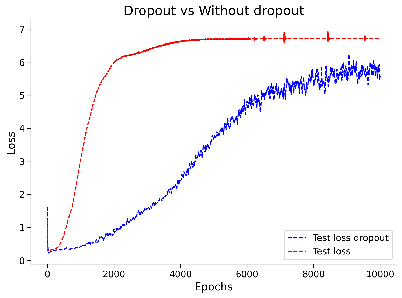
Plot the train and test losses with epoch
Show code cell source
# @markdown Plot the train and test losses with epoch

plt.figure()
plt.plot(test_loss_dp, label='Test loss dropout', c='blue', ls='dashed')
plt.plot(test_loss, label='Test loss', c='red', ls='dashed')
plt.ylabel('Loss')
plt.xlabel('Epochs')
plt.title('Dropout vs Without dropout')
plt.legend()
plt.show()
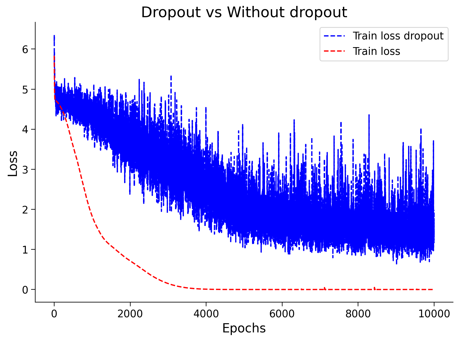
Plot the train and test losses with epoch
Show code cell source
# @markdown Plot the train and test losses with epoch

plt.figure()
plt.plot(train_loss_dp, label='Train loss dropout', c='blue', ls='dashed')
plt.plot(train_loss, label='Train loss', c='red', ls='dashed')
plt.ylabel('Loss')
plt.xlabel('Epochs')
plt.title('Dropout vs Without dropout')
plt.legend()
plt.show()
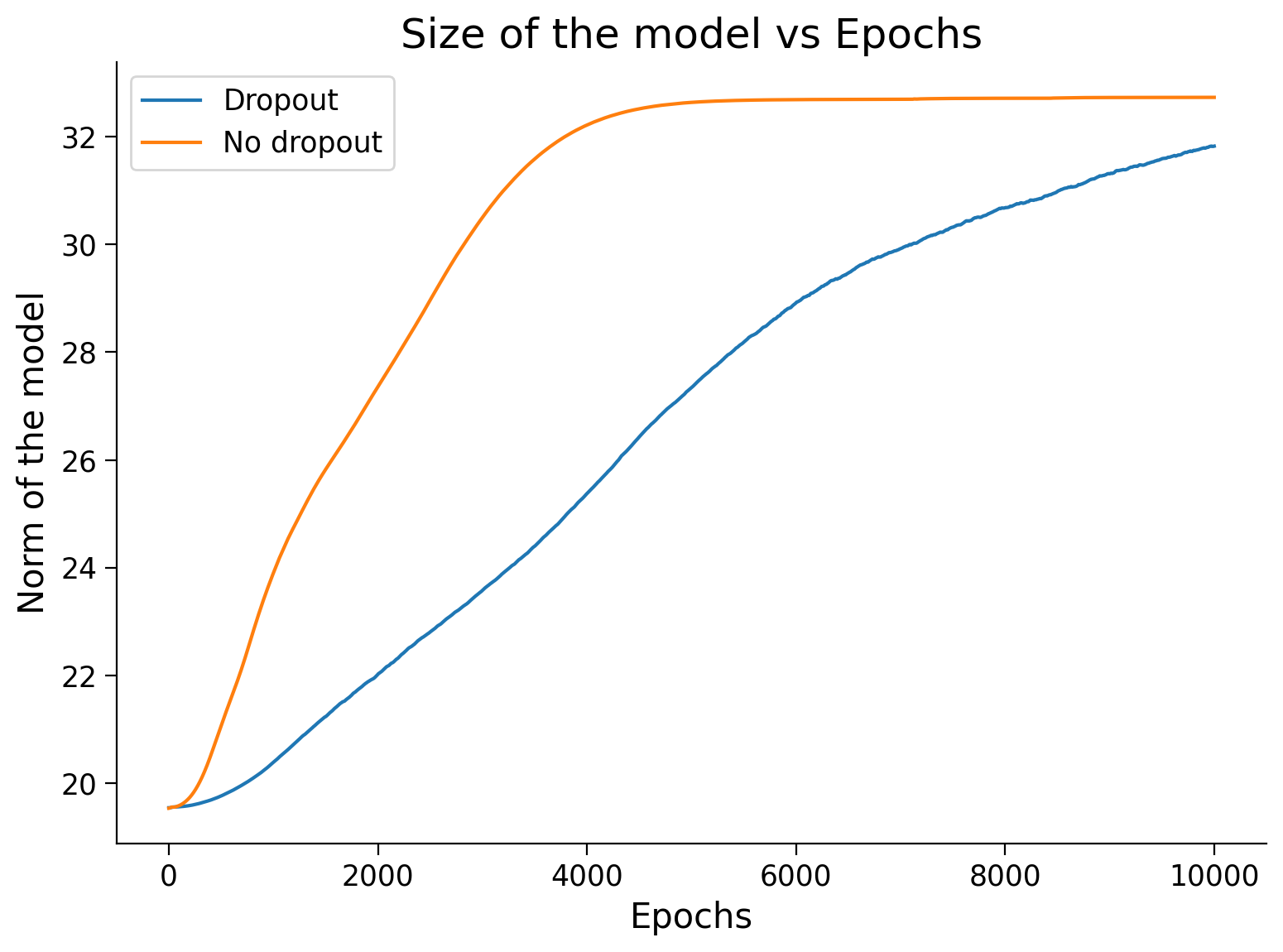
Plot model weights with epoch
Show code cell source
# @markdown Plot model weights with epoch
plt.figure()
plt.plot(model_norm_dp, label='Dropout')
plt.plot(model_norm, label='No dropout')
plt.ylabel('Norm of the model')
plt.xlabel('Epochs')
plt.legend()
plt.title('Size of the model vs Epochs')
plt.show()
Think 2.1!: Dropout#
Do you think this (with dropout) performed better than the initial model (without dropout)?
Submit your feedback#
Show code cell source
# @title Submit your feedback
content_review(f"{feedback_prefix}_Dropout_Discussion")
Section 2.1: Dropout Implementation Caveats#
Dropout is used only during training. However, the complete model weights are used during testing, so it is vital to use the
model.eval()method before testing the model.Dropout reduces the capacity of the model during training, and hence as a general practice, wider networks are used when using dropout. If you are using a dropout with a random probability of 0.5, you might want to double the number of hidden neurons in that layer.
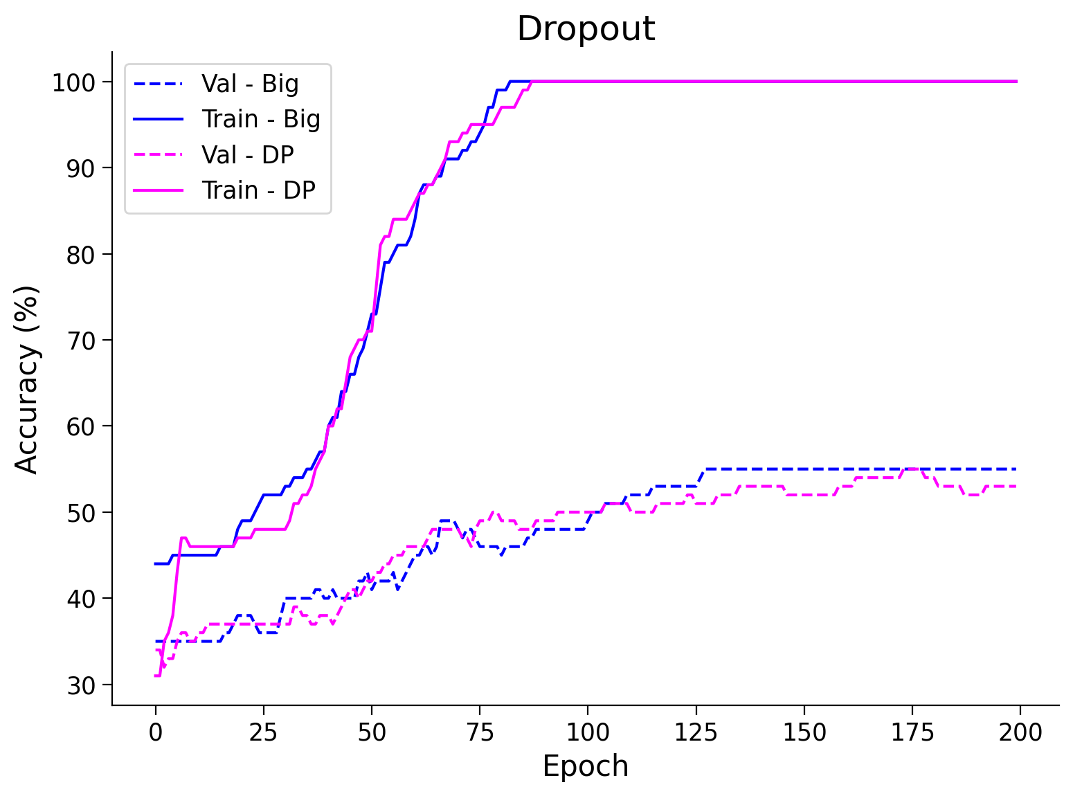
Now, let’s see how dropout fares on the “Animal Faces” dataset. We first modify the existing model to include dropout and then train it.
class AnimalNetDropout(nn.Module):
  """
  Network Class - Animal Faces with following structure
  nn.Linear(3*32*32, 248) + leaky_relu(self.dropout1(self.fc1(x))) # First fully connected layer with 0.5 dropout
  nn.Linear(248, 210) + leaky_relu(self.dropout2(self.fc2(x))) # Second fully connected layer with 0.3 dropout
  nn.Linear(210, 3) # Final fully connected layer
  """

  def __init__(self):
    """
    Initialize parameters of AnimalNetDropout

    Args:
      None

    Returns:
      Nothing
    """
    super(AnimalNetDropout, self).__init__()
    self.fc1 = nn.Linear(3*32*32, 248)
    self.fc2 = nn.Linear(248, 210)
    self.fc3 = nn.Linear(210, 3)
    self.dropout1 = nn.Dropout(p=0.5)
    self.dropout2 = nn.Dropout(p=0.3)

  def forward(self, x):
    """
    Forward pass of AnimalNetDropout

    Args:
      x: torch.tensor
        Input features

    Returns:
      x: torch.tensor
        Output/Predictions
    """
    x = x.view(x.shape[0], -1)
    x = F.leaky_relu(self.dropout1(self.fc1(x)))
    x = F.leaky_relu(self.dropout2(self.fc2(x)))
    x = self.fc3(x)
    output = F.log_softmax(x, dim=1)
    return output
# Set the arguments
args = {
    'test_batch_size': 1000,
    'epochs': 200,
    'lr': 5e-3,
    'batch_size': 32,
    'momentum': 0.9,
    'device': DEVICE,
    'log_interval': 100
}

# Initialize the model
set_seed(seed=SEED)
model = AnimalNetDropout()

# Train the model with Dropout
val_acc_dropout, train_acc_dropout, _, model_dp = main(args,
                                                       model,
                                                       train_loader,
                                                       val_loader,
                                                       img_test_dataset)

# Initialize the BigAnimalNet model
set_seed(seed=SEED)
model = BigAnimalNet()

# Train the model
val_acc_big, train_acc_big, _, model_big = main(args,
                                                model,
                                                train_loader,
                                                val_loader,
                                                img_test_dataset)


# Train and Test accuracy plot
plt.figure()
plt.plot(val_acc_big, label='Val - Big', c='blue', ls='dashed')
plt.plot(train_acc_big, label='Train - Big', c='blue', ls='solid')
plt.plot(val_acc_dropout, label='Val - DP', c='magenta', ls='dashed')
plt.plot(train_acc_dropout, label='Train - DP', c='magenta', ls='solid')
plt.title('Dropout')
plt.ylabel('Accuracy (%)')
plt.xlabel('Epoch')
plt.legend()
plt.show()
Random seed 2021 has been set.
Random seed 2021 has been set.
Think 2.2! Dropout caveats#
When do you think dropouts can perform bad and do you think their placement within a model matters?
Submit your feedback#
Show code cell source
# @title Submit your feedback
content_review(f"{feedback_prefix}_Dropout_Caveats_Discussion")
Section 3: Data Augmentation#
Time estimate: ~15 mins
Video 3: Data Augmentation#
Submit your feedback#
Show code cell source
# @title Submit your feedback
content_review(f"{feedback_prefix}_Data_Augmentation_Video")
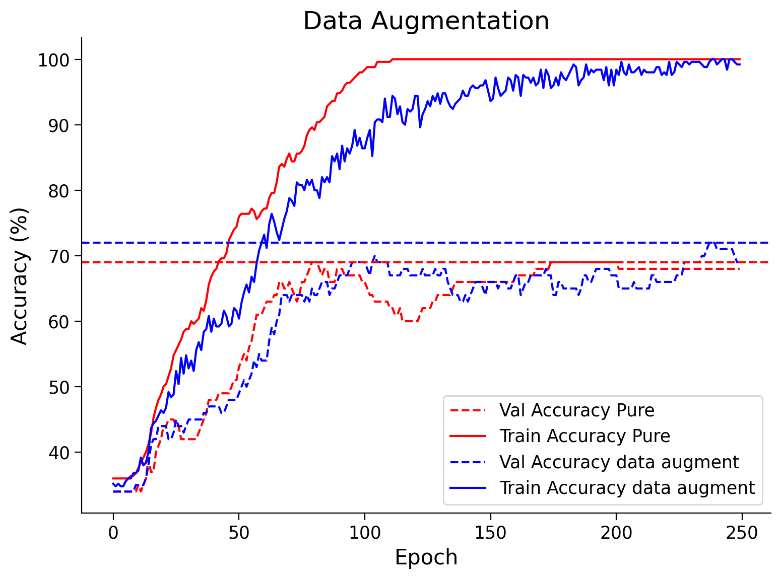
Data augmentation is often used to increase the number of training samples. Now we will explore the effects of data augmentation on regularization. Here regularization is achieved by adding noise into training data after every epoch.
PyTorch’s torchvision module provides a few built-in data augmentation techniques, which we can use on image datasets. Some of the techniques we most frequently use are:
Random Crop
Random Rotate
Vertical Flip
Horizontal Flip
Data Loader without Data Augmentation#
Show code cell source
# @markdown ####  Data Loader without Data Augmentation

# For reproducibility
g_seed = torch.Generator()
g_seed.manual_seed(SEED)


train_transform = transforms.Compose([
     transforms.ToTensor(),
     transforms.Normalize((0.5, 0.5, 0.5), (0.5, 0.5, 0.5))
     ])
data_path = pathlib.Path('.')/'afhq' # Using pathlib to be compatible with all OS's
img_dataset = ImageFolder(data_path/'train', transform=train_transform)

# Splitting dataset
img_train_data, img_val_data,_ = torch.utils.data.random_split(img_dataset, [250,100,14280])

# Creating train_loader and Val_loader
train_loader = torch.utils.data.DataLoader(img_train_data,
                                           batch_size=batch_size,
                                           num_workers=2,
                                           worker_init_fn=seed_worker,
                                           generator=g_seed)
val_loader = torch.utils.data.DataLoader(img_val_data,
                                         batch_size=1000,
                                         num_workers=2,
                                         worker_init_fn=seed_worker,
                                         generator=g_seed)
Define a DataLoader using torchvision.transforms, which randomly augments the data for us. For more info, see here.
# Data Augmentation using transforms
new_transforms = transforms.Compose([
                                     transforms.RandomHorizontalFlip(p=0.1),
                                     transforms.RandomVerticalFlip(p=0.1),
                                     transforms.ToTensor(),
                                     transforms.Normalize((0.5, 0.5, 0.5),
                                                          (0.5, 0.5, 0.5))
                                     ])

data_path = pathlib.Path('.')/'afhq'  # Using pathlib to be compatible with all OS's
img_dataset = ImageFolder(data_path/'train', transform=new_transforms)
# Splitting dataset
new_train_data, _,_ = torch.utils.data.random_split(img_dataset,
                                                    [250, 100, 14280])

# For reproducibility
g_seed = torch.Generator()
g_seed.manual_seed(SEED)

# Creating train_loader and Val_loader
new_train_loader = torch.utils.data.DataLoader(new_train_data,
                                               batch_size=batch_size,
                                               worker_init_fn=seed_worker,
                                               generator=g_seed)
# Set the arguments
args = {
    'epochs': 250,
    'lr': 1e-3,
    'momentum': 0.99,
    'device': DEVICE,
}

# Initialize the model
set_seed(seed=SEED)
model_aug = AnimalNet()

# Train the model
val_acc_dataaug, train_acc_dataaug, param_norm_dataaug, _ = main(args,
                                                                 model_aug,
                                                                 new_train_loader,
                                                                 val_loader,
                                                                 img_test_dataset)
# Initialize the model
set_seed(seed=SEED)
model_pure = AnimalNet()

val_acc_pure, train_acc_pure, param_norm_pure, _, = main(args,
                                                         model_pure,
                                                         train_loader,
                                                         val_loader,
                                                         img_test_dataset)


# Train and Test accuracy plot
plt.figure()
plt.plot(val_acc_pure, label='Val Accuracy Pure',
         c='red', ls='dashed')
plt.plot(train_acc_pure, label='Train Accuracy Pure',
         c='red', ls='solid')
plt.plot(val_acc_dataaug, label='Val Accuracy data augment',
         c='blue', ls='dashed')
plt.plot(train_acc_dataaug, label='Train Accuracy data augment',
         c='blue', ls='solid')
plt.axhline(y=max(val_acc_pure), c='red', ls='dashed')
plt.axhline(y=max(val_acc_dataaug), c='blue', ls='dashed')
plt.title('Data Augmentation')
plt.ylabel('Accuracy (%)')
plt.xlabel('Epoch')
plt.legend()
plt.show()
Random seed 2021 has been set.
Random seed 2021 has been set.
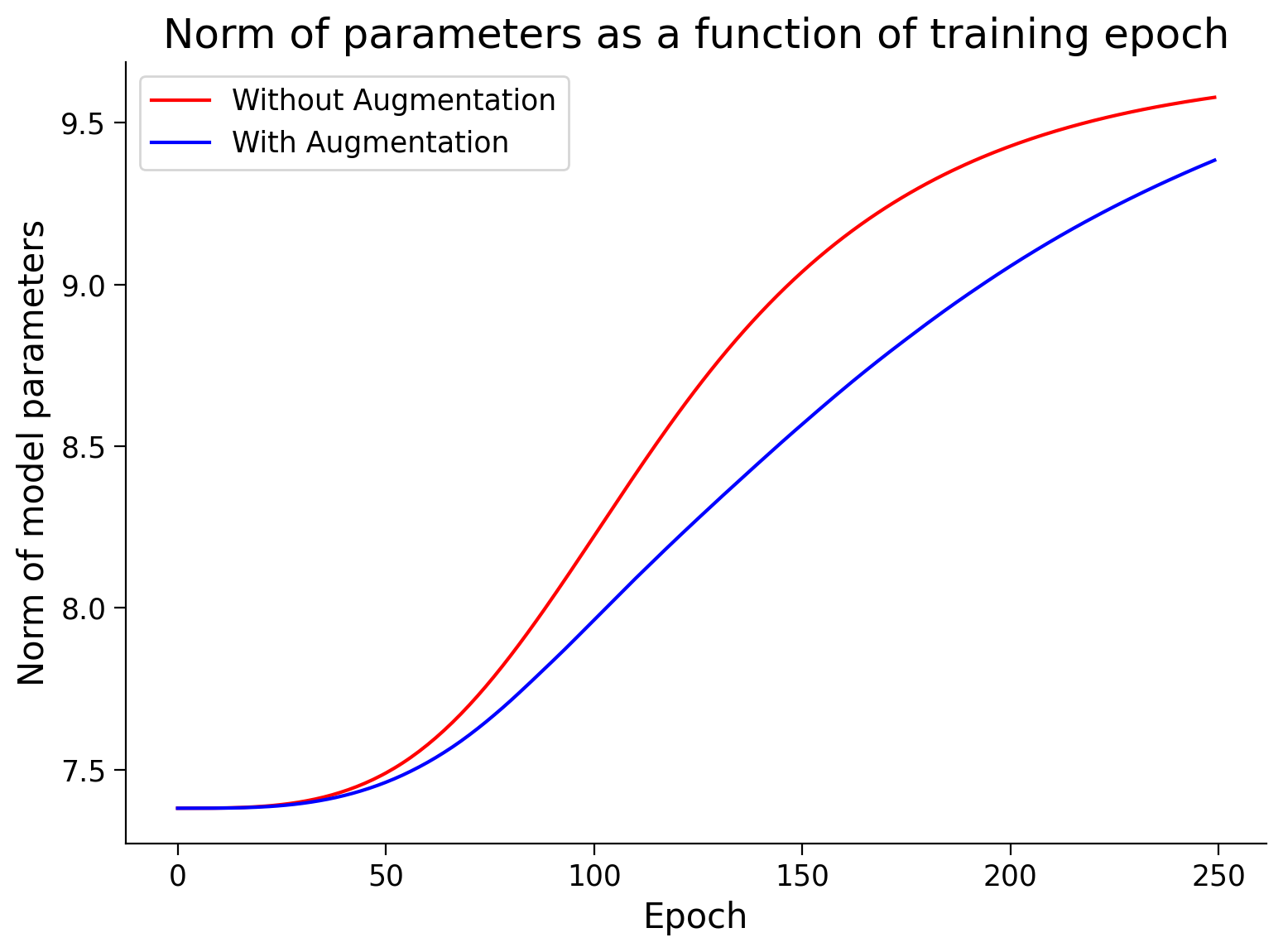
# Plot together: without and with augmentation
plt.figure()
plt.plot([i.cpu().numpy().item() for i in param_norm_pure],
         c='red', label='Without Augmentation')
plt.plot([i.cpu().numpy().item() for i in param_norm_dataaug],
         c='blue', label='With Augmentation')
plt.title('Norm of parameters as a function of training epoch')
plt.xlabel('Epoch')
plt.ylabel('Norm of model parameters')
plt.legend()
plt.show()
Think 3.1!: Data Augmentation#
Can you think of more ways of augmenting the training data? (Think of other problems beyond object recognition.)
Submit your feedback#
Show code cell source
# @title Submit your feedback
content_review(f"{feedback_prefix}_Data_Augmentation_Discussuion")
Think! 3.2!: Overparameterized vs. Small NN#
Why is it better to regularize an overparameterized ANN than to start with a smaller one? Think about the regularization methods you know. Each group should have a 10 min discussion.
Submit your feedback#
Show code cell source
# @title Submit your feedback
content_review(f"{feedback_prefix}_Overparameterized_vs_Small_NN_Discussuion")
Section 4: Stochastic Gradient Descent#
Time estimate: ~20 mins
Video 4: SGD#
Submit your feedback#
Show code cell source
# @title Submit your feedback
content_review(f"{feedback_prefix}_SGD_Video")
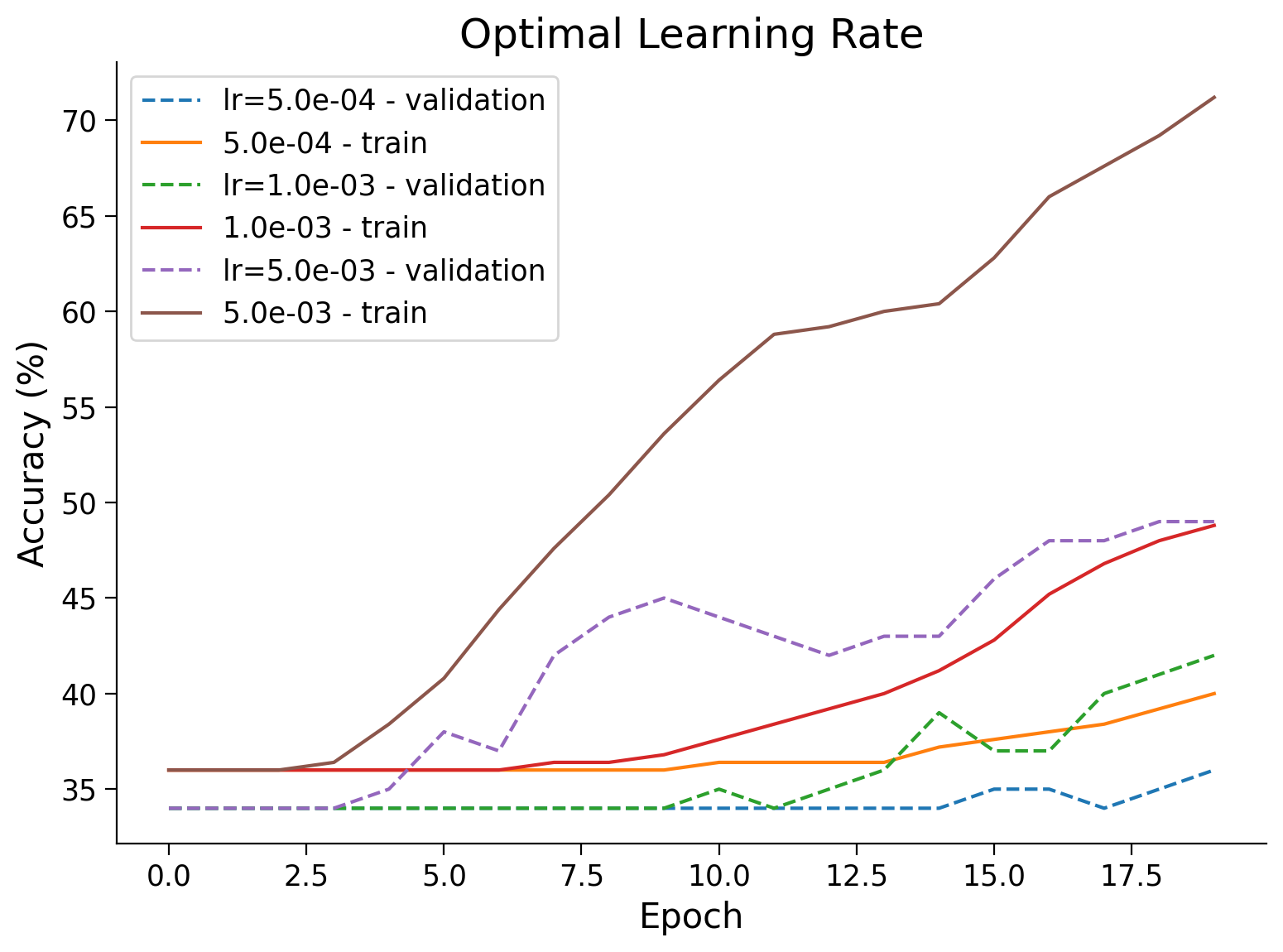
Section 4.1: Learning Rate#
In this section, we will see how the learning rate can act as a regularizer while training a neural network. In summary:
Smaller learning rates regularize less and slowly converge to deep minima.
Larger learning rates regularize more by missing local minima and converging to broader, flatter minima, which often generalize better.
But beware, a very large learning rate may result in overshooting or finding a bad local minimum.
In the block below, we will train the AnimalNet model with different learning rates and see how that affects the regularization.
Generating Data Loaders#
Show code cell source
# @markdown #### Generating Data Loaders

# For reproducibility
g_seed = torch.Generator()
g_seed.manual_seed(SEED)

batch_size = 128
train_transform = transforms.Compose([
     transforms.ToTensor(),
     transforms.Normalize((0.5, 0.5, 0.5), (0.5, 0.5, 0.5))
     ])

data_path = pathlib.Path('.')/'afhq' # Using pathlib to be compatible with all OS's
img_dataset = ImageFolder(data_path/'train', transform=train_transform)
img_train_data, img_val_data, = torch.utils.data.random_split(img_dataset, [11700,2930])

full_train_loader = torch.utils.data.DataLoader(img_train_data,
                                                batch_size=batch_size,
                                                num_workers=2,
                                                worker_init_fn=seed_worker,
                                                generator=g_seed)
full_val_loader = torch.utils.data.DataLoader(img_val_data,
                                              batch_size=1000,
                                              num_workers=2,
                                              worker_init_fn=seed_worker,
                                              generator=g_seed)

test_transform = transforms.Compose([
     transforms.ToTensor(),
     transforms.Normalize((0.5, 0.5, 0.5), (0.5, 0.5, 0.5))
     ])
img_test_dataset = ImageFolder(data_path/'val', transform=test_transform)
# With dataloaders: img_test_loader = DataLoader(img_test_dataset, batch_size=batch_size,shuffle=False, num_workers=1)
classes = ('cat', 'dog', 'wild')
# Set the arguments
args = {
    'test_batch_size': 1000,
    'epochs': 20,
    'batch_size': 32,
    'momentum': 0.99,
    'device': DEVICE
}

learning_rates = [5e-4, 1e-3, 5e-3]
acc_dict = {}

for i, lr in enumerate(learning_rates):
  # Initialize the model
  set_seed(seed=SEED)
  model = AnimalNet()
  # Learning rate
  args['lr'] = lr
  # Train the model
  val_acc, train_acc, param_norm, _ = main(args,
                                           model,
                                           train_loader,
                                           val_loader,
                                           img_test_dataset)
  # Store the outputs
  acc_dict[f'val_{i}'] = val_acc
  acc_dict[f'train_{i}'] = train_acc
  acc_dict[f'param_norm_{i}'] = param_norm
Random seed 2021 has been set.
Random seed 2021 has been set.
Random seed 2021 has been set.
Plot Train and Validation accuracy (Run me)
Show code cell source
# @markdown Plot Train and Validation accuracy (Run me)
plt.figure()
for i, lr in enumerate(learning_rates):
  plt.plot(acc_dict[f'val_{i}'], linestyle='dashed',
          label=f'lr={lr:0.1e} - validation')
  plt.plot(acc_dict[f'train_{i}'], label=f'{lr:0.1e} - train')

  print(f"Maximum Test Accuracy obtained with lr={lr:0.1e}: {max(acc_dict[f'val_{i}'])}")

plt.title('Optimal Learning Rate')
plt.ylabel('Accuracy (%)')
plt.xlabel('Epoch')
plt.legend()
plt.show()
Maximum Test Accuracy obtained with lr=5.0e-04: 36.0
Maximum Test Accuracy obtained with lr=1.0e-03: 42.0
Maximum Test Accuracy obtained with lr=5.0e-03: 49.0
Plot parametric norms (Run me)
Show code cell source
# @markdown Plot parametric norms (Run me)
plt.figure()
for i, lr in enumerate(learning_rates):
  plt.plot([i.cpu().numpy().item() for i in acc_dict[f'param_norm_{i}']],
           label=f'lr={lr:0.2e}')
plt.legend()
plt.xlabel('Epoch')
plt.ylabel('Parameter norms')
plt.show()

In the model above, we observe something different from what we expected. Why do you think this is happening?
Section 5: Hyperparameter Tuning#
Time estimate: ~5 mins
Video 5: Hyperparameter tuning#
Submit your feedback#
Show code cell source
# @title Submit your feedback
content_review(f"{feedback_prefix}_Hyperparameter_tuning_Video")
Hyperparameter tuning is often tricky and time-consuming, and it is a vital part of training any Deep Learning model to give good generalization. There are a few techniques that we can use to guide us during the search.
Grid Search: Try all possible combinations of hyperparameters
Random Search: Randomly try different combinations of hyperparameters
Coordinate-wise Gradient Descent: Start at one set of hyperparameters and try changing one at a time, accept any changes that reduce your validation error
Bayesian Optimization / Auto ML: Start from a set of hyperparameters that have worked well on a similar problem, and then do some sort of local exploration (e.g., gradient descent) from there.
There are many choices, like what range to explore over, which parameter to optimize first, etc. Some hyperparameters don’t matter much (people use a dropout of either 0.5 or 0.2, but not much else). Others can matter a lot more (e.g., size and depth of the neural net). The key is to see what worked on similar problems.
One can automate the process of tuning the network architecture using the so called Neural Architecture Search (NAS). NAS designs new architectures using a few building blocks (Linear, Convolutional, Convolution Layers, etc.) and optimizes the design based on performance using a wide range of techniques such as Grid Search, Reinforcement Learning, Gradient Descent, Evolutionary Algorithms, etc. This obviously requires very high computing power. Read this article to learn more about NAS.
Think! 5: Overview of regularization techniques#
Which regularization technique today do you think had the most significant effect on the network? Why might do you think so? Can you apply all of the regularization methods on the same network?
Submit your feedback#
Show code cell source
# @title Submit your feedback
content_review(f"{feedback_prefix}_Overview_of_regularization_techniques_Discussion")
Summary#
Congratulations! You have finished the first week of NMA-DL!
In this tutorial, you learned more regularization techniques, i.e., L1 and L2 regularization, Dropout, and Data Augmentation. Finally, you have seen that the learning rate of SGD can act as a regularizer. An interesting paper can be found here.
Continue to the Bonus material on Adversarial Attacks if you have time left!
Bonus: Adversarial Attacks#
Time estimate: ~15 mins
Video 6: Adversarial Attacks#
Submit your feedback#
Show code cell source
# @title Submit your feedback
content_review(f"{feedback_prefix}_Adversarial_Attacks_Bonus_Video")
Designing perturbations to the input data to trick a machine learning model is called an “adversarial attack”. These attacks are an inevitable consequence of learning in high dimensional space using complex decision boundaries. Depending on the application, these attacks can be very dangerous.
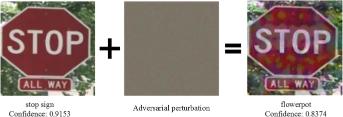
Hence, we need to build models which can defend against such attacks. One possible way to do it is by regularizing the networks, which smooths the decision boundaries. A few ways of building models robust to such attacks are:
Defensive Distillation: Models trained via distillation are less prone to such attacks as they are trained on soft labels as there is an element of randomness in the training process.
Feature Squeezing: Identifies adversarial attacks for online classifiers whose model is being used by comparing the model’s prediction before and after squeezing the input.
SGD: You can also pick weight to minimize what the adversary is trying to maximize via SGD.
Read more about adversarial attacks here.